Chapter 1
Maxwell's Equations and Electromagnetic Fields
1.1 Introduction
1.1.1 Maxwell's Equations (1865)
The governing equations of electromagnetism
| E | electric field, describes the force felt by a (stationary)
charge q: F = q E |
| B | magnetic field, describes the force felt by a current |
| i.e. a moving charge (velocity v): F = q v∧B |
Thus the Lorentz Force (on charge q) is
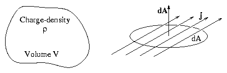
Figure 1.1:
Charge density is local charge per
unit volume. Current density is current per unit area.
| ρ | electric charge density (Coulombs/m3).
Total charge Q = ∫V ρd3x |
| j | electric current density (Coulombs/s/m2) |
| Current crossing area element dA is j . dA
Coulomb/s = Amps. |
[Note. Sometimes the first Maxwell equation is called Gauss's
rather than Coulomb's Law.]
1.1.2 Historical Note
Much scientific controversy in 2nd half of 19th century concerned
question of whether E, B were `real' physical quantities
of science or else mere mathematical conveniences for expressing
the forces that charges exert on one another. English science
(Faraday, Maxwell) emphasized the fields; German mostly the
act-at-a-distance. Since ∼ 1900 this question has been
regarded as settled in favor of the fields. And modern
physics, if anything, tends to regard the field as more
fundamental than the particle.
1.1.3 Auxiliary Fields and Electromagnetic Media
Electromagnetic texts often discuss two additional "auxiliary"
fields D the "electric displacement" and H
the "magnetic intensity" which account for dielectric and
magnetic properties of materials. These fields are not fundamental
and introduce unnecessary complication and possible confusion
for most of our topics. Therefore we will avoid them as much
as possible. For the vacuum, ϵ0 E
= D and
B
= μ0 H.
1.1.4 Units
Historically there were two (or more!) different
systems of units, one defining the quantity of charge in terms
of the force between two stationary charges (the
"Electrostatic" units) and one defining it in terms of forces
between (chargeless) currents (the "Electromagnetic"
system). Electrostatic units are based on Coulomb's law
∇. E
= ρ/ϵ0 and electromagnetic units on
the (steady-state version of) Ampere's law ∇∧B
=μ0 j. The quantities 1/ϵ0 and μ0 are
therefore fundamentally calibration factors that determine the
size of the unit charge. Choosing one or other of them to be 4π
amounts to choosing electrostatic or electromagnetic units.
However, with the unification of electromagnetism, and the
subsequent realization that the speed of light is a fundamental
constant, it became clear that the units of electromagnetism
ought to be defined in terms of only one of these laws and the speed
of light.
Therefore the "System Internationale" SI (or sometimes MKSA)
units adopts the electromagnetic definition because it can be
measured most easily, but with a different μ0, as
follows.
"One Ampere is that current which, when flowing in two
infinitesimal parallel wires 1m apart produces a force of
2 ×10⁻⁷ Newtons per meter of their length."
An Amp is one Coulomb per second. So this defines the unit
of charge. We will show later that this definition amounts to
defining
|
μ0 = 4π×10−7 (Henry/meter) |
| (1.3) |
and that because the ratio of electromagnetic to electrostatic
units is c2
|
ϵ0 = |
1
c2 μ0
|
= 8.85 ×10⁻¹² (Farad/meter) |
| (1.4) |
μ0 is called the "permeability of free space".
ϵ0 is called the "permittivity of free space".
[See J.D. Jackson 3rd Ed, Appendix for a detailed discussion.]
1.2 Vector Calculus and Notation
Electromagnetic quantities include vector fields E,B etc. and
so EM draws heavily on vector calculus.
∇ is shorthand for a vector operator (gradient)
|
∇ϕ = | ⎛
⎝
|
∂ϕ
∂x
|
, |
∂ϕ
∂y
|
, |
∂ϕ
∂z
| ⎞
⎠
|
= |
∂ϕ
∂xi
|
(suffix notation) |
| (1.5) |
giving a vector gradient from a scalar field ϕ.
∇ can also operate on vector fields by scalar (.) or vector
(∧) multiplication.
1.2.1 Divergence
|
∇. E= |
∂Ex
∂x
|
+ |
∂Ey
∂y
|
+ |
∂Ez
∂z
|
= |
∂Ei
∂xi
|
|
| (1.6) |
1.2.2 Curl
|
∇∧E= | ⎛
⎝
|
∂Ez
∂y
|
− |
∂Ey
∂z
|
, |
∂Ex
∂z
|
− |
∂Ez
∂x
|
, |
∂Ey
∂x
|
− |
∂Ex
∂y
| ⎞
⎠
|
= ϵijk |
∂Ek
∂xj
|
|
| (1.7) |
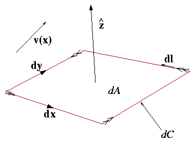
1.2.3 Volume Integration
d3x is shorthand for dxdydz = dV, the volume element.
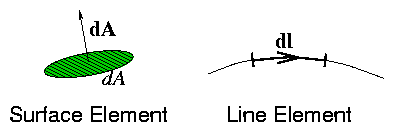
Figure 1.2:
Elements for surface and line integrals.
1.2.4 Surface Integration
The surface element dA or often dS is a vector normal to the element.
1.2.5 Line (Contour) Integration
Line element dl.
1.2.6 The Meaning of divergence: ∇.
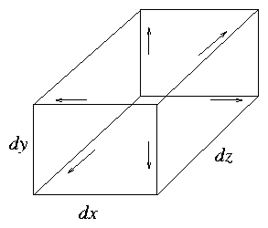
Figure 1.3:
Cartesian volume element.
| |
[vx (x + dx/2) − vx (x−dx/2)] dydz+ |
|
| |
| |
[vy (y + dy/2) − vy (y−dy/2) ] dzdx+ |
|
| |
| |
[vz (z + dz/2) − vz (z−dz/2)] dxdy |
|
|
| | (1.11) |
| |
dxdydz | ⎡
⎣
|
dvx
dx
|
+ |
dvy
dy
|
+ |
dvz
dz
| ⎤
⎦
|
|
|
|
| |
|
So for this elemental volume:
|
| ⌠
⌡
|
dS
|
v. dA= | ⌠
⌡
|
dV
|
∇. v d3x |
| (1.12) |
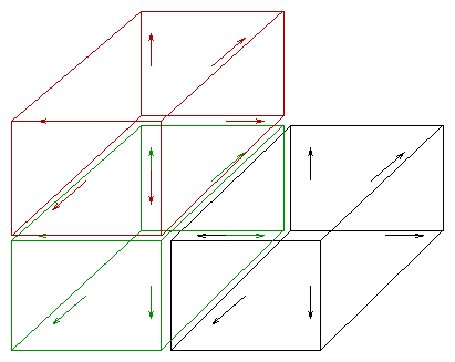
Figure 1.4:
Adjacent faces cancel out in
the sum of divergence from many elements.
|
| ⌠
⌡
|
S
|
v. dA= | ⌠
⌡
|
V
|
∇. v d3x |
| (1.13) |
for any volume V with surface S, and arbitrary vector
field v.
This is Gauss's Theorem.
1.2.7 The Meaning of Curl: ∇∧
Figure 1.5:
Rectangular surface element with axes
chosen such that the normal is in the
z-direction.
| |
|
|
v(x,y−dy/2). dx + v(x+dx/2,y) . dy |
| | (1.14) |
| |
|
|
v(x,y+dy/2) . (−dx)+ v(x−dx/2,y) . (−dy) |
| |
| |
|
|
−dvxdx + dvydy = | ⎛
⎝
|
∂vy
∂x
|
− |
∂vx
∂y
| ⎞
⎠
|
dxdy |
| |
| |
|
| | (1.15) |
|
So integral v.d l around element is equal to the curl
scalar-product area element.
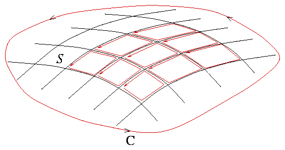
Figure 1.6:
Arbitrary surface may be divided into
the sum of many rectangular elements. Adjacent edge integral
contributions cancel.
|
| ⌠
(⎜)
⌡
|
C
|
v.dl= | ⌠
⌡
|
S
|
( ∇∧v) . dA |
| (1.16) |
This is Stokes' Theorem.
1.3 Electrostatics and Gauss' Theorem
Gauss's theorem is the key to understanding electrostatics in
terms of Coulomb's Law ∇.E
= ρ/ ϵ0.
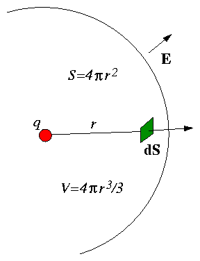
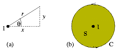
1.3.1 Point Charge q
Apply Gauss's Theorem to a sphere surrounding q
Figure 1.7:
Spherical volume, V over
which we perform an integral of Coulomb's law to deduce
E.
|
| ⌠
⌡
|
S
|
E. dA= | ⌠
⌡
|
V
|
∇. E d3x = | ⌠
⌡
|
V
|
|
ρ
ϵ0
|
d3x = |
q
ϵ0
|
. |
| (1.17) |
But by spherical symmetry E must be in radial direction and
Er has magnitude constant over the sphere.
Hence
∫S E. dA
= ∫S ErdA = Er ∫S dA = Er 4πr2.
Thus
|
Er = |
q
4πϵ0 r2
|
i.e. E
= |
q
4πϵ0
|
|
r
r3
|
. |
| (1.19) |
Consequently, force on a second charge at distance r is
Coulomb's inverse-square-law of electrostatic force.
1.3.2 Spherically Symmetric Charge ρ(r)
Notice that point-charge derivation depended only on symmetry.
So for a distributed charge-density that is symmetric argument
works just the same i.e.
|
where now q = | ⌠
⌡
|
V
|
ρ d3x = | ⌠
⌡
|
r
0
|
ρ(r) 4πr2dr . |
| (1.22) |
Electric field due to a spherically symmetric charge density
is equal to that of a point charge of magnitude equal to the
total charge within the radius, placed at the spherical
center.
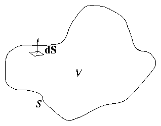
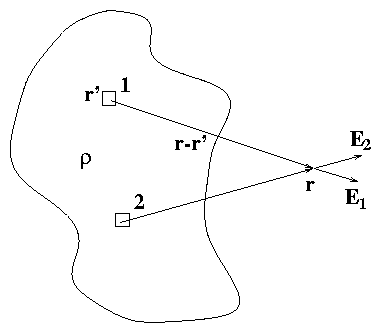
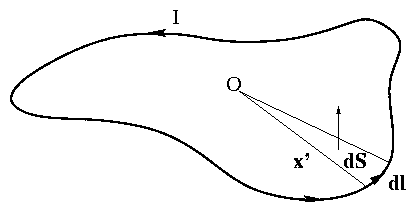
1.3.3 Arbitrary Charge Distribution
If there is no specific symmetry Gauss's Theorem still applies:
Figure 1.8:
Arbitrary volume for Gauss's Theorem.
|
| ⌠
⌡
|
S
|
E. dA= | ⌠
⌡
|
V
|
∇. E d3x = | ⌠
⌡
|
V
|
|
ρ
ϵ0
|
d3x = |
q
ϵ0
|
|
| (1.23) |
q is the total charge (integral of charge density) over the volume.
∫S E. dA is the total flux of electric field across
the surface S.
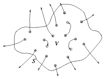
1.3.4 Intuitive Picture
Figure 1.9:
Intuitive picture of charges and
field-lines.
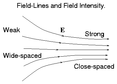
Figure 1.10:
Spacing of field-lines is
inversely proportional to field-strength.
1.3.5 Electric Potential (for static problems
[(∂)/(∂t)] → 0)
In the static situation there is no induction and Faraday's law
becomes ∇∧E
= 0.
By the way, this equation could also be derived from the inverse-square-law
by noting that
Figure 1.11:
Each element contributes an
irrotational component to
E. Therefore the total
E is irrotational.
so by the linearity of the ∇∧ operator the sum (integral)
of all Electric field contributions from any charge distribution is
curl-free "irrotational":
|
∇∧ | ⌠
⌡
|
|
ρ(r′)
4πϵ0
|
|
r−r′
|r−r′|3
|
d3r′ = 0 |
| (1.25) |
[This shows that the spherical symmetry argument only works in the
absence of induction · B would define a preferred direction;
asymmetric!]
For any vector field E, ∇∧E
= 0 is a necessary
and sufficient condition that E can be written as the gradient
of a scalar E
= − ∇ϕ.
Necessary
|
( ∇∧∇ϕ)z = |
∂
∂x
|
|
∂ϕ
∂y
|
− |
∂
∂y
|
|
∂ϕ
∂x
|
= 0 (et sim x, y) . |
| (1.26) |
Curl of a gradient is zero.
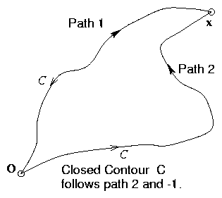
Sufficient (prove by construction)
Figure 1.12:
Two different paths from 0
to
x construct a closed contour when one is reversed.
|
| ⌠
(⎜)
⌡
|
C
|
E. dl= |
Path 2
|
− |
Path 1
|
= | ⌠
⌡
|
S
|
∇∧E. dS |
= 0
by hypothesis.
|
|
| (1.27) |
So ∇∧E
= 0 ⇒ ∫oxE. dl is
independent of chosen path, i.e. it defines a
unique3
quantity.
Call it −ϕ(x).
Consider ∇ϕ defined as the limit of δϕ between
adjacent points.
|
− ∇ϕ = ∇ | ⎛
⎝
| ⌠
⌡
|
x
|
E. dl | ⎞
⎠
|
= E . |
| (1.28) |
Many electrostatic problems are most easily solved in terms of
the electric potential ϕ because it is a scalar (so easier).
Governing equation:
| |
|
| | (1.29) |
| |
|
|
|
∂2
∂x2
|
+ |
∂2
∂y2
|
+ |
∂2
∂x2
|
is the "Laplacian" operator |
| | (1.30) |
| |
|
| ∇2 ϕ = |
−ρ
ϵ0
|
"Poisson′s Equation". |
| | (1.31) |
|
1.3.6 Potential of a Point Charge [General Potential Solution]
One can show by direct differentiation that
So by our previous expression E
= [q/(4 πϵ0)] [(r)/(r3)] we can identify
as the potential of a charge q (at the origin x
=0).
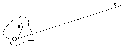
1.3.7 Green Function for the Laplacian
For a linear differential operator, L, mathematicians define
something called "Green's function" symbolically by the equation
If we can solve this equation in general, then solutions to
can be constructed for arbitrary ρ as
|
ϕ(x) = | ⌠
⌡
|
G(x, x′) ρ(x′) d3x′ |
| (1.36) |
because of the (defining) property of the δ-function
|
| ⌠
⌡
|
f(x′) δ(x−x′) d3x′ = f(x) . |
| (1.37) |
When L is the Laplacian, ∇2, the Green function is
This fact may be derived directly from the solution for the
potential for a point charge. Indeed, a point charge is exactly
the delta-function situation whose solution is the Green function.
In other words, the charge density for a point charge of magnitude
q at position x′ is
so the point-charge potential,
namely,
is the solution of the equation:
Consequently, solution of Poisson's equation can be written as
the integral of the Green function:
|
ϕ(x) = | ⌠
⌡
|
| ⎛
⎝
|
−ρ( x′)
ϵ0
| ⎞
⎠
|
| ⎛
⎝
|
−1
4π|x−x′|
| ⎞
⎠
|
d3 x′ = | ⌠
⌡
|
|
ρ(x′)
4 πϵ0
|
|
d3x′
|x− x′|
|
. |
| (1.42) |
Informally, the smooth charge distribution ρ can be
approximated as the sum (→ ∫) of many point charges
ρ(x′) d3x′, and the potential is the sum of their
contributions.
1.3.8 Boundary Conditions
Strictly speaking, our solution of Poisson's equation is not unique.
We can always add to ϕ a solution of the homogeneous
(Laplace) equation ∇2ϕ = 0.
The solution only becomes unique when boundary conditions are
specified. The solution
|
ϕ(x) = | ⌠
⌡
|
|
ρ( x′)
4 πϵ0
|
|
d3x′
|x− x′|
|
|
| (1.43) |
is correct when the boundary conditions are that
no applied external field.
In practice most interesting electrostatic calculations involve specific
boundaries. A big fraction of the work is solving Laplace's equation
with appropriate boundary conditions. These are frequently the specification
of ϕ on (conducting) surfaces. The charge density on the conductors
is rarely specified initially.
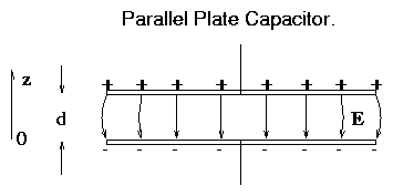
1.3.9 Parallel Plate Capacitor
Figure 1.13:
The parallel-plate capacitor.
Solution ϕ = a − Ez a,E const.
Hence electric field is
E
= E ∧z.
Notice how this arises purely from the
translational invariance of ϕ( [d/dx] = [d/dy] = 0 ).
Choose z=0 as one plate of capacitor. Other at z = d.
Choose ϕ(z=0) = 0: reference potential, making a = 0.
Potential of other plate: V = ϕ(d) = −Ed.
The question: how
much charge per unit area is there on the plates when the field is
E?
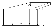
Figure 1.14:
Elemental volume for
calculating charge/field relationship.
| |
|
| |
| |
|
| ⌠
⌡
|
V
|
|
ρ
ϵ0
|
d3x = |
Q
ϵ0
|
= |
1
ϵ0
|
σ A |
| | (1.46) |
|
Hence
Therefore if the total area is A, the total charge
Q, and the
voltage V between plates are related by
And the coefficient [(ϵ0A)/d] is called capacitance, C.
Notice our approach:
- Solve Laplace's equation by choosing coordinates consistent
with problem symmetry.
- Obtain charge using Gauss's law to an appropriate
trial volume.
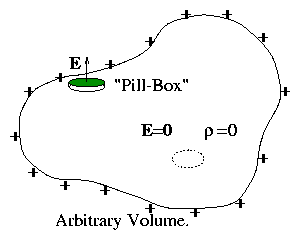
1.3.10 Charge on an arbitrary conductor
Consider a conductor, electrostatically charged.
Figure 1.15:
Arbitrary-shaped conductor possesses
only surface charges related to the local normal field.
So E is zero, anywhere inside because of conductivity.
Choose any volume internally: E
= 0 ⇒ ∇. E = 0 ⇒ρ = 0. There is no internal charge. It all resides
on surface.
At the surface there is an E just outside.
E is perpendicular to surface ds because surface is
an equipotential (& E
= − ∇ϕ).
Hence applying Gauss's law to a pill box
| |
| ⌠
⌡
|
V
|
∇. E d3x = | ⌠
⌡
|
S
|
E. dS |
|
|
| |
| |
= | ⌠
⌡
|
|
ρ
ϵ0
|
d3 x = | ⌠
⌡
|
|
σ
ϵ0
|
ds |
|
|
| | (1.49) |
|
where σ = surface charge density
Hence σ = ϵ0 E.
Of course, in this general case E (= Enormal) is
not uniform on the surface but varies from place to place.
Again procedure would be: solve ϕ externally from ∇2ϕ = 0;
then deduce σ; rather than the other way around.
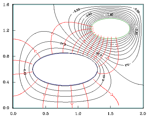
1.3.11 Visualizing Electric Potential and Field
Figure 1.16:
Contours of potential and
corresponding field-lines (marked with arrows). Only the field-lines
emanating from the larger elliptical conductor are drawn.
1.3.12 Complex Potential Representation 2-D
In charge-free region, ∇. E
= 0 ⇒ ∇2 ϕ = 0.
This causes there to be an intimate relationship between field-lines and
ϕ-contours. In 2 dimensions this relationship allows complex
analysis to be used to do powerful analysis of potential problems.
Consider a complex function f(z) = ϕ(z) + i ψ(z)
where z = x + iy is the complex argument with real and imaginary
parts x & y; and f has real and imaginary parts ϕ & ψ.
f is "analytic" if there exists a well defined complex derivative
[df/dz] (which is also analytic), defined in the usual
way as limz′→ z ( [(f( z′) − f ( z ))/(z′− z )] ) .
In order for this limit to be the same no matter what direction (x,y)
it is taken in, f must satisfy the "Cauchy-Riemann relations"
|
|
∂ϕ
∂x
|
= |
∂ψ
∂y
|
; |
∂ϕ
∂y
|
= − |
∂ψ
∂x
|
|
| (1.51) |
Which, by substitution imply ∇2ϕ = 0, ∇2ψ = 0,
and also
regarding x,y as 2-d coordinates. This shows that
- The real part of an analytic function solves ∇2ϕ = 0.
- The contours of the corresponding imaginary part, ψ,
then coincide
with the electric field-lines.
Finding complex representations of potential problems is one of the most
powerful analytic solution techniques. However, for practical
calculations, numerical solution techniques are now predominant.
1.4 Electric Current in Distributed Media
Ohms law, V = IR, relates voltage current and resistance for
a circuit or discrete element. However we often care not just about
the total current but about the current density
in finite-sized conductors (e.g. electromagnets).
This requires a local Ohm's law which is
where η is the medium's electric resistivity.
Often the conductivity σ = 1/η is used.
j = σE, (but I'll try to avoid confusion with
surface charge density σ).
Such a linear relationship applies in most metals.
1.4.1 Steady State Conduction
Conservation of charge can be written
so, in steady state, ∇. j = 0, i.e.
|
∇. | ⎛
⎝
|
1
η
|
E | ⎞
⎠
|
= ( E. ∇) |
1
η
|
+ |
1
η
|
∇. E= 0 |
| (1.55) |
If conductivity
is uniform (∇[1/(η)] = 0) or invariant
along E, we therefore have ∇. E
= 0 ⇒ ρ = 0.
"Uniform conductivity conductors acquire zero volume charge
density in steady state".
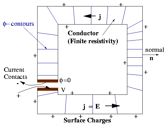
1.4.2 Conductor Boundary Conditions (Steady Currents)
Figure 1.17:
A distributed conductor of finite
conductivity, carrying current.
inside conductor, while outside we have
surface charge density.
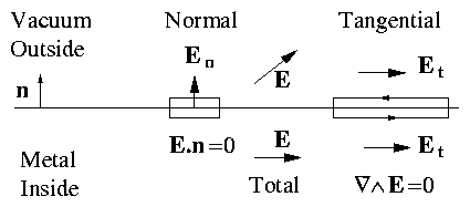
Normal components
Figure 1.18:
Boundary conditions across a
conductor/vacuum (or insulator) interface.
|
En|inside = 0 [ En ]insideoutside = σ/ϵ0 |
| (1.58) |
Tangential components
In particular, for solving ∇2 ϕ = 0 inside uniform η
conductor, at conductor boundary:
unlike the usual electrostatic B.C. ϕ = given.
At electrical contacts ϕ given might be appropriate.
A general approach to solving a distributed steady-current
problem with uniform-η media:
- Solve Laplace's equation ∇2ϕ = 0 inside
conductors using Dirichlet (ϕ-given) or possibly inhomogeneous
Neumann (∇ϕ|n = given) BC's at contacts and
∇ϕ. n = 0 at insulating boundaries.
- Solve Laplace's equation ∇2 ϕ = 0 outside
conductors using ϕ = given (Dirichlet) B.C. with the ϕ
taken from the internal solution.
1.5 Magnetic Potential
Magnetic field has zero divergence ∇. B
= 0.
For any vector field4
B, ∇. B
= 0 is a necessary and sufficient
condition that B can be written as the curl of a vector potential
B
= ∇∧A.
1.5.1 ∇.B
=0 Necessary
| |
|
|
|
∂
∂x
|
| ⎛
⎝
|
∂Az
∂y
|
(z)
|
− |
∂Ay
∂z
|
(y)
| ⎞
⎠
|
|
| | (1.61) |
| |
|
|
|
∂
∂y
|
| ⎛
⎝
|
∂Ax
∂z
|
(x)
|
− |
∂Az
∂x
|
(z)
| ⎞
⎠
|
|
| | (1.62) |
| |
|
|
∂
∂z
|
| ⎛
⎝
|
∂Ay
∂x
|
(y)
|
− |
∂Ax
∂y
|
(x)
| ⎞
⎠
|
= 0 |
| | (1.63) |
|
So only divergenceless fields can be represented.
1.5.2 ∇.B
=0 Sufficient (outline proof by construction)
Consider the quantity
|
K(x) = | ⌠
⌡
|
|
B( x′)
4 π|x− x′|
|
d3 x′ , |
| (1.64) |
a vector constructed from the integral of each Cartesian component
of B. Applying our knowledge of the Green function solution
of Poisson's equation, we know:
Vector operator theorem (for any v):
|
∇∧( ∇∧v ) = ∇( ∇. v ) − ∇2 v . |
| (1.66) |
Hence
|
B= − ∇2 K = ∇∧( ∇∧K) − ∇( ∇. K ) |
| (1.67) |
We have proved Helmholtz's theorem that any vector field can be
represented as the sum of grad + curl.]
When ∇. B
= 0 and |B| → 0 (fast enough) as
|x| → ∞, one can show that ∇. K = 0
and so we have constructed the required vector potential
|
A= ∇∧K = ∇∧ | ⌠
⌡
|
|
B( x′)
4 π
|
|
d3x′
|x− x′|
|
. |
| (1.68) |
Notice that we have constructed A such that
∇. A
= 0. However A is undetermined from B because
we can add to it the gradient of an arbitrary scalar without
changing B, since ∇∧∇χ = 0. So in
effect we can make ∇. A equal any desired quantity
ψ(x) by adding to A ∇χ such that
∇2χ = ψ.
Choosing ∇. A is known as choosing a "Gauge"
∇. A
= 0 is the "Coulomb Gauge".
1.5.3 General Vector Potential Solution (Magnetostatic)
Static Ampere's law ∇∧B
= μ0 j.
Now
| |
|
| |
| |
|
| ∇( ∇. A) − ∇2 A= − ∇2 A (Coulomb Gauge). |
| | (1.69) |
|
Hence Cartesian components of A are solutions of Poisson equation
Using our general solution of Poisson's equation (see eq 1.38):
|
A(x) = |
μ0
4π
|
| ⌠
⌡
|
|
j ( x′)
|x− x′|
|
d3x′ |
| (1.71) |
Resulting B:
| |
|
|
∇∧A= |
μ0
4π
|
| ⌠
⌡
|
∇∧ |
j ( x′)
|x− x′|
|
d3x′ |
| |
| |
|
|
μ0
4π
|
| ⌠
⌡
|
− j (x′) ∧∇ |
1
|x− x′|
|
d3x′ = |
μ0
4π
|
| ⌠
⌡
|
|
j( x′) ∧( x− x′)
|x− x′|3
|
d3x′ |
| | (1.72) |
|
This is the distributed-current version of the law of
Biot and Savart
(dating from ∼ 1820).
For a wire carrying current I the integral over volume j is
replaced by the integral I dl i.e.
|
B= |
μ0
4π
|
| ⌠
⌡
|
− |
( x− x′)
|x− x′|3
|
∧j d3 x = |
μ0
4π
|
| ⌠
⌡
|
− |
( x−x′)
|x− x′|3
|
∧I dl . |
| (1.73) |
The Biot-Savart law gives us a direct means to calculate B
by integrating over j(x′), numerically if necessary.
However this integration brute-force method is excessively
computationally intensive and if symmetries are present in the problem
we can use them to simplify.
1.5.4 Cartesian Translational Symmetry (2-d x,y)
Figure 1.19:
(a) The coordinates with respect
to an infinite straight filament carrying current I, and (b) the contour
and surface for use with Ampere's law.
|
| ⌠
⌡
|
S
|
( ∇∧B) . ds = | ⌠
⌡
|
C
|
B. dl = | ⌠
⌡
|
S
|
μ0 j . ds = μ0 I |
| (1.74) |
By symmetry (∫)C B. dl = 2πr Bθ
So
Also Br = 0 by applying Gauss's Theorem to a volume (of unit
length in z-dir)
|
0 = | ⌠
⌡
|
V
|
∇. B d3x = | ⌠
⌡
|
S
|
B. dS = 2πr Br |
| (1.76) |
by symmetry.
Thus Maxwell's equations immediately show us what the 2-d Green
function solving ∇∧B
= μ0 I ∧z δ(x−x′) is
Any general j(x,y) can be handled by 2-d integration using this
function.
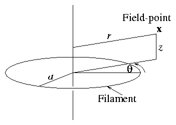
1.5.5 Cylindrical Symmetry (Circular Loops with common axis)
If there exist cylindrical coordinates (r, θ, z) such that
∂/∂θ = 0, j = j ∧θ.
Then by symmetry A
= Aθ ∧θ, Bθ = 0.
This situation turns out to be soluble analytically but only in terms
of the special functions known as Elliptic Integrals.
Figure 1.20:
Cylindrical Coordinates near a circular
current-carrying filament.
then
|
Aθ (r,z) = |
μ0
4 π
|
2 |
⎛
√
|
|
| ⎡
⎣
|
( 2 − k2 ) K(k) − 2 E(k)
k
| ⎤
⎦
|
|
| (1.79) |
where
|
k2 ≡ |
4 ra
( r + a )2 + z2
|
|
| (1.80) |
and K, E are the complete elliptical integrals of the first
and second kind.
This general form is so cumbersome that it does not make general
analytic calculations tractable but it makes numerical evaluation
easier by using canned routines for K(k) & E(k).
On axis (r=0) the field is much simpler
|
B= B |
^
z
|
= |
μ0 I
4 π
|
|
2 πa2
( z2 + a2 )3/2
|
|
^
z
|
. |
| (1.81) |
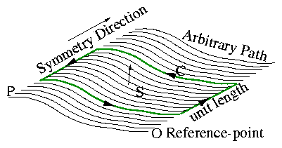
1.5.6 General Property of Symmetry Situations: Flux Function
When there is a symmetry direction, the component of B
perpendicular to that direction can be expressed in terms of a
"flux function".
The magnetic flux between two positions is defined as the B-field
flux crossing a surface spanning the gap (per unit length if
translational).
Figure 1.21:
Path from a reference point to a
field point defines a surface to which Stokes' theorem is applied, in
a situation of translational symmetry.
is well defined.
For translational (∧z) symmetry, a consequence is
This arises because
|
ψ = | ⌠
⌡
|
S
|
B. dS = | ⌠
⌡
|
∇∧A. dS = Az(P) − Az(0) |
| (1.84) |
So really ψ is identical to the z-component of the
vector potential and
| |
|
|
Bz |
^
z
|
+ ∇∧ | ⎛
⎝
|
Az |
^
z
| ⎞
⎠
|
= Bz |
^
z
|
+ B⊥ |
| |
| |
|
| | (1.85) |
| |
|
| |
|
B⊥ is the part of the field perpendicular to ∧z.
There could also be Bz.
For cylindrical symmetry some more variations arise from
curvilinear coordinate system. There are even other symmetries, for
example helical!
1.6 Electromagnetism and Magnets
1.6.1 Simple Solenoid
Figure 1.22:
Idealized long solenoid magnet coil.
|
0 = ∇. B= |
1
r
|
|
∂
∂r
|
r Br + |
=0
|
Bθ + |
=0
|
Bz |
| (1.86) |
So
|
rBr = const. and hence Br = 0 . |
| (1.87) |
Also
|
∇∧B= | ⎛
⎝
|
1
r
|
|
∂
∂r
|
r Bθ | ⎞
⎠
|
|
^
z
|
+ | ⎛
⎝
|
− |
∂
∂r
|
Bz | ⎞
⎠
|
|
^
θ
|
= μ0 j (steady) |
| (1.88) |
Inside the bore of the magnet, j = 0
so
|
rBθ = const. and hence Bθ = 0 . |
| (1.89) |
(actually if jz = 0 everywhere then Bθ = 0 everywhere, as
may be seen immediately from the Biot-Savart law). Also
|
|
∂Bz
∂r
|
= 0 and hence Bz = const . |
| (1.90) |
Use the surface and bounding curve shown and write
|
| ⌠
⌡
|
S
|
μ0 j . dS = | ⌠
⌡
|
S
|
∇∧B. ds = | ⌠
(⎜)
⌡
|
C
|
B. dl |
| (1.91) |
So μ0 × current per unit length (denoted
Jθ) gives
|
μ0 Jθ = Bz inside − Bz outside |
| (1.92) |
But (by same approach) if B = 0 at infinity Bz outside = 0.
So, inside
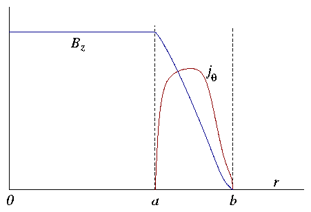
Profile of field in coil:
Figure 1.23:
The field profile within the
conductor region of the coil depends on the current-density profile.
|
Bzb − Bza = − | ⌠
⌡
|
b
a
|
μ0 jθ dr = − μ0 Jθ . |
| (1.95) |
(as before).
Notice that all this is independent of coil thickness (b−a).
Coils are usually multi-turn so
where n is turns per unit length, I is current in each turn.
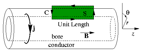
1.6.2 Solenoid of Arbitrary Cross-Section
Figure 1.24:
Solenoid of arbitrary cross-section.
Consider Biot-Savart Law, expressed as vector potential:
|
A(r) = |
μ0
4π
|
| ⌠
⌡
|
|
j ( r′)
|r− r′|
|
d3 r′ . |
| (1.99) |
If currents all flow in azimuthal direction, i.e. jz = 0,
then Az = 0.
|
⇒ Bx = By = 0 (everywhere.) |
| (1.100) |
Then integral form of Ampere's law is still
where Jp is total current in azimuthal direction per unit length.
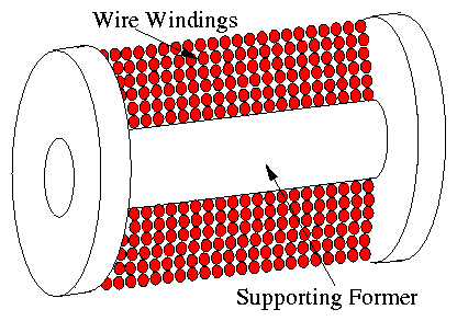
1.6.3 Coil Types
(a) Wire (Filament):
Figure 1.25:
Section through a wire-wound
magnet coil.
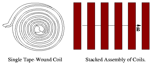
(b) Tape wound:
Figure 1.26:
Tape-wound coils are stacked to
produce a solenoid.
(c) Pancake:
Similar to tape but using square or rectangular conductor.
(Fewer turns/coil).
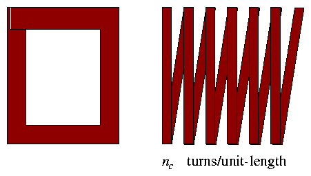
(d) Plate Coils:
Figure 1.27:
A picture-frame type plate coil
and the configuration of a solenoid.
1.6.4 Magnetic Dipole
Figure 1.28:
Currents localized to a small
region close to the origin, with the field point far away.
|
A(x) = |
μ0
4π
|
| ⌠
⌡
|
|
j ( x′)
|x− x′|
|
d3x′ |
| (1.102) |
can be approximated by writing
|
|
1
|x− x′|
|
= |
1
(x2 − 2 x. x′+ x′2 )1/2
|
≈ |
1
|x|
|
| ⎛
⎝
|
1 + |
x. x′
|x|2
|
+ ... | ⎞
⎠
|
|
| (1.103) |
so
|
A ≅ |
μ0
4π
|
|
1
|x|
|
| ⎡
⎣
| ⌠
⌡
|
j ( x′) d3x′+ |
1
|x|2
|
| ⌠
⌡
|
x. x′ j ( x′) d3x′ | ⎤
⎦
|
. |
| (1.104) |
Now we convert these integrals into more convenient expressions
using ∇. j = 0. Actually the first one is zero.
This follows immediately from the identity
|
∇. ( j x) = x( ∇. j ) +( j . ∇) x= j |
| (1.105) |
(which uses ∇x
= I i.e. ∂xi/∂xj = δij, and ∇. j = 0).
So
|
| ⌠
⌡
|
j d3x′ = | ⌠
⌡
|
∇′. ( j x′) d3x′ = | ⌠
⌡
|
S
|
x′j . dS = 0 , |
| (1.106) |
for any surface S that encloses all currents so that j = 0 on
S. An intuitive way to see this is that ∫jd3x is the
average velocity of charges, and must be zero.
The second term is simplified using the same identity but being
careful to distinguish between x and x′,
and using notation ∇′ to denote the gradient operator
that operates on x′, j(x′), not
on x.
| |
|
|
| ⌠
⌡
|
( x. x′) ∇′. ( j x′) d3x′ |
| |
| |
|
|
| ⌠
⌡
|
∇′. ( j x′( x. x′)) − x′j . ∇′( x′. x) d3x′ |
| |
| |
|
|
− | ⌠
⌡
|
x′j. ( ∇′x′) . x d3x′ |
| |
| |
|
| − | ⌠
⌡
|
x′j . I . x d3x′ = − | ⌠
⌡
|
x′( j . x) d3 x′ |
| | (1.107) |
|
But
|
x∧( x′∧j ) = ( j . x) x′− ( x. x′) j . |
| (1.108) |
So
|
| ⌠
⌡
|
x∧( x′∧j ) d3x′ = −2 | ⌠
⌡
|
x. x′j d3 x′ , |
| (1.109) |
by the integral relation just proved. [This identity is true for
any x].
Therefore our approximation for A is
|
A( x) = − |
μ0
4π
|
|
x
|x|3
|
∧ | ⎛
⎝
|
1
2
|
| ⌠
⌡
|
x′∧j ( x′) d3 x′ | ⎞
⎠
|
|
| (1.110) |
or
where the Magnetic Dipole Moment of the localized
current distribution is
We have derived this expression for an arbitrary j distribution;
but if the localized current is a loop current filament,
Figure 1.29:
Current-carrying loop
integration to give dipole moment.
|
m = |
1
2
|
| ⌠
⌡
|
x′∧j d3x′ = |
1
2
|
| ⌠
⌡
|
x∧I dl . |
| (1.113) |
If the loop is planar,
where ds
is the element of surface. So m is (current ×
area) for a planar filament.
The magnetic field is obtained from B
= ∇∧A
|
B= |
μ0
4 π
|
| ⎡
⎣
|
3 |
x
|x|
|
| ⎛
⎝
|
x
|x|
|
. m | ⎞
⎠
|
− m | ⎤
⎦
|
|
1
|x|3
|
|
| (1.115) |
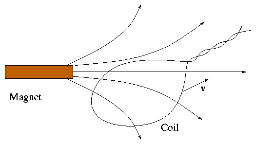
1.6.5 Revisionist History of Electromagnetic Induction
Michael Faraday first showed the effect of induction: a transient
current can be induced in one circuit by changes in another. This
was ∼ 1830. [Faraday knew no mathematics beyond the idea of
proportionality EMF ∝ rate of change of B-flux].
Suppose history had been different and we knew only the Lorentz
force law:
we could have "proved" the necessity of induction by "pure
thought".
Assume Galilean Invariance: physical laws must be invariant
under changes to moving coordinate systems x′ = x −vt,
t′ = t.
[Universally assumed in Faraday's time. Einstein doesn't come
till 1905!]
Consider a rigid (wire) circuit moved past a magnet:
Figure 1.30:
A rigid coil moving past a
steady magnet.
as it is dragged through the magnetic field. The electric field in the
rest frame of the magnet is zero. And the total
electromotive force (integrated force per unit charge) round the
entire circuit is
|
|
1
q
|
| ⌠
(⎜)
⌡
|
C
|
F . dl = | ⌠
(⎜)
⌡
|
C
|
v∧B. dl |
| (1.118) |
This is generally a non-zero quantity.
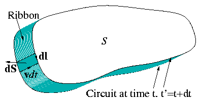
In fact, this quantity can be transformed on the basis of purely geometrical
considerations.
Figure 1.31:
Surface elements in the
application of Gauss's theorem to succeeding instants of time.
| |
|
|
| ⌠
⌡
|
V
|
∇. B d3 x = | ⌠
⌡
|
Stotal
|
B. dS = | ⌠
⌡
|
S′
|
− | ⌠
⌡
|
S
|
+ | ⌠
⌡
|
ribbon
|
B. ds |
| |
| |
|
|
| ⌠
⌡
|
S′
|
B. dS − | ⌠
⌡
|
S
|
B. dS + | ⌠
⌡
|
B. ( dl∧vdt ) |
| |
| |
|
| | (1.119) |
|
[where dΦ is change in flux].
So
|
|
d Φ
dt
|
= − | ⌠
(⎜)
⌡
|
C
|
( v∧B) . dl . |
| (1.120) |
(pure geometry when ∂B/∂t = 0).
This equation can alternatively be obtained algebraically by writing
|
|
d Φ
dt
|
= | ⌠
⌡
|
|
dB
dt
|
. dS = | ⌠
⌡
|
( v. ∇) B. dS |
| (1.121) |
and using
|
∇∧( B∧v) = ( v. ∇) B+ (∇.v) B− (B.∇) v− ( ∇. B) v = ( v. ∇) B . |
| (1.122) |
So
|
|
dΦ
dt
|
= | ⌠
⌡
|
∇∧( B∧v) .dS = | ⌠
(⎜)
⌡
|
C
|
( B∧v) . dS |
| (1.123) |
Anyway EMF is
|
|
1
q
|
| ⌠
(⎜)
⌡
|
C
|
F . dl = | ⌠
(⎜)
⌡
|
C
|
(v∧B) . dS = − |
dΦ
dt
|
|
| (1.124) |
Now we consider the whole situation when the frame of reference
is changed to one in which the circuit is stationary and the magnet
is moving.
By Galilean invariance the total EMF is the same, and
|
|
1
q
|
| ⌠
(⎜)
⌡
| F . dl = − |
dΦ
dt
|
|
| (1.125) |
But now v
= 0, and instead B is changing so
In this case also the Lorentz force on the charges is
|
F = q ( E + v∧B) = q E (since v
=0) |
| (1.127) |
There has to be an electric field in this frame of reference.
And also
|
|
1
q
|
| ⌠
(⎜)
⌡
| F . dl = | ⌠
(⎜)
⌡
| E . dl = − |
dΦ
dt
|
= − | ⌠
⌡
|
|
∂B
∂t
|
. dS |
| (1.128) |
Apply Stokes' theorem to the E . dl integral:
|
| ⌠
⌡
|
S
|
| ⎡
⎣
|
∇∧E + |
∂B
∂t
| ⎤
⎦
|
. dS = 0 . |
| (1.129) |
But this integral has to be zero for all S (and C) which can be true only
if its integrand is everywhere zero:
"Faraday's" Law (expressed in differential form) (which Faraday
understood intuitively but could not have formulated in math)
1.6.6 Inductance
Suppose we have a set of circuits with currents Ii (i = 1 ... N).
These are inductively coupled if the current in one gives rise to flux
linking the others. Because Ampere's law is linear (B ∝ j),
the flux linking circuit j from current Ii is proportional to
Ii. Consequently, the total flux linking circuit j can be written
(Summation over Ii) different currents.
M is a matrix. The element Mij is an inductance
between currents i and j..
Its units are
|
|
flux
current
|
↔ |
Wb
A
|
↔ Henrys . |
| (1.132) |
The electromotive force or voltage Vj induced in the j'th
circuit is then:
|
Vj = |
d
dt
|
Φj = |
∑
i
|
Mji |
⋅
I
|
i
|
. |
| (1.133) |
For the simplest case N=1 circuit. Mii → L
the self inductance
It can be shown from Maxwell's equations that Mij is
symmetric.