<?xml version="1.0"?>
<!DOCTYPE html    PUBLIC "-//W3C//DTD XHTML 1.1 plus MathML 2.0//EN"
           "http://www.w3.org/Math/DTD/mathml2/xhtml-math11-f.dtd">
<html xmlns="http://www.w3.org/1999/xhtml">
<head>
<meta name="GENERATOR" content="TtM 4.12" />
 <style type="text/css">
 div.p { margin-top: 7pt; }
 span.roman {font-family: serif; font-style: normal; font-weight: normal;} 
</style>
 <style type="text/css">
 .tiny {font-size:30%;}
 .scriptsize {font-size:xx-small;}
 .footnotesize {font-size:x-small;}
 .smaller {font-size:smaller;}
 .small {font-size:small;}
 .normalsize {font-size:medium;}
 .large {font-size:large;}
 .larger {font-size:x-large;}
 .largerstill {font-size:xx-large;}
 .huge {font-size:300%;}
 </style>
<title>chap9.xml</title>
</head>
<body><div>
<table width="100%"><tr><td>
 <a href="index.xml">HEAD</a></td><td align="right">
 <a href="chap8.xml">PREVIOUS
</a></td></tr></table>
 <a id="tth_chAp9"></a><h1>
Chapter 9 <br />Energy-Resolved Diffusive Transport</h1>

<div class="p"><!----></div>
When there are strong processes that drive the velocity distribution
function away from equilibrium<a 
id="non-equilibrium90530"></a>, it is generally
important to account for the full distribution of velocities of
particles to understand their transport. Sources of particles with
kinetic energy substantially higher than the typical (e.g.&nbsp;thermal)
energy will have this effect. Examples include all sorts of
<em>reactions</em>; for example the chemical reactions<a 
id="reactions90531"></a>
that occur in combustion, or, as we will address in this chapter, the
nuclear reactions that involve neutrons.<a href="footnote.xml#tthFtNtAEH" id="tthFrefAEH"><math xmlns="http://www.w3.org/1998/Math/MathML">
<mrow>
<msup><mrow></mrow><mrow><mn>47</mn></mrow>
</msup>
</mrow></math></a>

<div class="p"><!----></div>
 <a id="tth_sEc9.1"></a><h2>
9.1&nbsp;&nbsp;Collisions of Neutrons</h2>

<div class="p"><!----></div>
Neutrons experience no net electric or magnetic forces, because they
are uncharged, and usually gravity is ignorable; so in Boltzmann's
equation the term proportional to the acceleration <math xmlns="http://www.w3.org/1998/Math/MathML">
<mrow><mi mathvariant="bold-italic">a</mi></mrow></math> can
usually be neglected. Self-collisions are also negligible. It is the
background matter through which the neutrons<a 
id="neutron91532"></a> are moving that
provides the targets with which the neutrons collide. It can be taken
to consist of practically stationary atoms. 

<div class="p"><!----></div>
Collisions give the crucial terms in Boltzmann's equation. They arise
from a whole host of different nuclear species, and the relevant
cross-sections<a 
id="cross-section91533"></a> have very strong dependence on
neutron kinetic energy (or equivalently speed, <math xmlns="http://www.w3.org/1998/Math/MathML">
<mrow><mi>v</mi></mrow></math>). We generally sum
over all the relevant species to give appropriate total source and
sink rates per unit phase-space volume. In addition to the sink of
neutrons, <math xmlns="http://www.w3.org/1998/Math/MathML">
<mrow><mo>-</mo>
<msub><mrow><mi mathvariant="italic">&Sigma;</mi></mrow><mrow><mi>t</mi></mrow>
</msub>
<mi mathvariant="italic">vf</mi></mrow></math> from all possible collisions, there are
sources arising from scattering, and from fission<a 
id="fission_reaction91534"></a>
reactions.<a href="footnote.xml#tthFtNtAEI" id="tthFrefAEI"><math xmlns="http://www.w3.org/1998/Math/MathML">
<mrow>
<msup><mrow></mrow><mrow><mn>48</mn></mrow>
</msup>
</mrow></math></a>  For
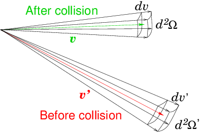
fission and scattering, as illustrated by Fig.&nbsp;<a href="chap9.xml#neutroncolnl">9.1</a>, we
consider an incoming neutron denoted with a prime (<math xmlns="http://www.w3.org/1998/Math/MathML">
<mrow><mo>'</mo></mrow></math>), having
velocity given by speed <math xmlns="http://www.w3.org/1998/Math/MathML">
<mrow><mi>v</mi><mo>'</mo></mrow></math>, and direction unit vector
<math xmlns="http://www.w3.org/1998/Math/MathML">
<mrow><mi mathvariant="bold-italic">&Omega;</mi><mo>'</mo></mrow></math><a 
id="direction_vector___bmOmega_91535"></a> (so <math xmlns="http://www.w3.org/1998/Math/MathML">
<mrow><mi mathvariant="bold-italic">v</mi><mo>'</mo><mo>=</mo><mi>v</mi><mo>'</mo><mi mathvariant="bold-italic">&Omega;</mi></mrow></math>) giving rise
to an outgoing (sourced) neutron with speed <math xmlns="http://www.w3.org/1998/Math/MathML">
<mrow><mi>v</mi></mrow></math>, and direction
<math xmlns="http://www.w3.org/1998/Math/MathML">
<mrow><mi mathvariant="bold-italic">&Omega;</mi></mrow></math>.  The 
"macroscopic cross-sections"<a 
id="macroscopic_cross-section91536"></a>  
are written
respectively <math xmlns="http://www.w3.org/1998/Math/MathML">
<mrow>
<msub><mrow><mi mathvariant="italic">&Sigma;</mi></mrow><mrow><mi>f</mi></mrow>
</msub>
</mrow></math> and <math xmlns="http://www.w3.org/1998/Math/MathML">
<mrow>
<msub><mrow><mi mathvariant="italic">&Sigma;</mi></mrow><mrow><mi>s</mi></mrow>
</msub>
</mrow></math>. They are functions of both
incoming and outgoing velocity, which is denoted <math xmlns="http://www.w3.org/1998/Math/MathML">
<mrow><mo stretchy="false">(</mo><mi>v</mi><mo>'</mo><mo>&rarr;</mo><mi>v</mi><mo>,</mo><mi mathvariant="bold-italic">&Omega;</mi><mo>'</mo><mo>&rarr;</mo><mi mathvariant="bold-italic">&Omega;</mi><mo stretchy="false">)</mo></mrow></math>.

<div class="p"><!----></div>
<a id="tth_fIg9.1">
</a>   <img src="figures/neutroncoln.png" alt="figures/neutroncoln.png" /><a id="neutroncoln">
</a>
  
<div style="text-align:center">Figure 9.1: Collisions give a source of particles in <math xmlns="http://www.w3.org/1998/Math/MathML">
<mrow>
<msup><mrow><mi mathvariant="italic">dvd</mi></mrow><mrow><mn>2</mn></mrow>
</msup>
<mi mathvariant="italic">&Omega;</mi></mrow></math> as a result
    of particles that (before the collision) are in
    <math xmlns="http://www.w3.org/1998/Math/MathML">
<mrow><mi mathvariant="italic">dv</mi><mo>'</mo>
<msup><mrow><mi>d</mi></mrow><mrow><mn>2</mn></mrow>
</msup>
<mi mathvariant="italic">&Omega;</mi><mo>'</mo></mrow></math>. Both induced fissions (weighted by the average
    neutron yield <math xmlns="http://www.w3.org/1998/Math/MathML">
<mrow><mi mathvariant="italic">&nu;</mi></mrow></math>) and scattering events contribute. The sink
    term in <math xmlns="http://www.w3.org/1998/Math/MathML">
<mrow>
<msup><mrow><mi mathvariant="italic">dvd</mi></mrow><mrow><mn>2</mn></mrow>
</msup>
<mi mathvariant="italic">&Omega;</mi></mrow></math> is the sum of all collisions that remove a
    particle from <math xmlns="http://www.w3.org/1998/Math/MathML">
<mrow>
<msup><mrow><mi mathvariant="italic">dvd</mi></mrow><mrow><mn>2</mn></mrow>
</msup>
<mi mathvariant="italic">&Omega;</mi></mrow></math>.<a id="neutroncolnl">
</a></div>

<div class="p"><!----></div>
Possible spatial dependence (on <math xmlns="http://www.w3.org/1998/Math/MathML">
<mrow><mi mathvariant="bold-italic">x</mi></mrow></math>) is implicit. Each fission
gives rise to an average number of outgoing neutrons <math xmlns="http://www.w3.org/1998/Math/MathML">
<mrow><mi mathvariant="italic">&nu;</mi></mrow></math> typically
greater than one, so for source the quantity required is actually
<math xmlns="http://www.w3.org/1998/Math/MathML">
<mrow><mi mathvariant="italic">&nu;</mi>
<msub><mrow><mi mathvariant="italic">&Sigma;</mi></mrow><mrow><mi>f</mi></mrow>
</msub>
</mrow></math>. Also, to calculate the source we must integrate over
all possible incoming velocities, for which we write the flux
density<a href="footnote.xml#tthFtNtAEJ" id="tthFrefAEJ"><math xmlns="http://www.w3.org/1998/Math/MathML">
<mrow>
<msup><mrow></mrow><mrow><mn>49</mn></mrow>
</msup>
</mrow></math></a>  as <math xmlns="http://www.w3.org/1998/Math/MathML">
<mrow><mi>v</mi><mo>'</mo><mi>f</mi><mo>'</mo></mrow></math> and the velocity element as
<math xmlns="http://www.w3.org/1998/Math/MathML">
<mrow>
<msup><mrow><mi>d</mi></mrow><mrow><mn>3</mn></mrow>
</msup>
<mi>v</mi><mo>'</mo><mo>=</mo>
<msup><mrow><mi>v</mi><mo>'</mo></mrow><mrow><mn>2</mn></mrow>
</msup>

<msup><mrow><mi>d</mi></mrow><mrow><mn>2</mn></mrow>
</msup>
<mi mathvariant="italic">&Omega;</mi><mo>'</mo><mi>&ensp;</mi><mi mathvariant="italic">dv</mi><mo>'</mo></mrow></math>. Thus Boltzmann's equation becomes the
neutron transport equation<a 
id="neutron_transport_equation91537"></a>:
<a id="neuttrans">
</a><br />
<table width="100%"><tr><td align="center">
    <math xmlns="http://www.w3.org/1998/Math/MathML">
    <mstyle displaystyle="true"><mrow>
<mtable>
<mtr><mtd columnalign="left"><mrow>
<mfrac><mrow><mo>&part;</mo><mi>f</mi></mrow>
<mrow><mo>&part;</mo><mi>t</mi></mrow>
</mfrac>
<mo>+</mo><mi>v</mi><mi mathvariant="bold-italic">&Omega;</mi><mo>.</mo>
<mfrac><mrow><mo>&part;</mo><mi>f</mi></mrow>
<mrow><mo>&part;</mo><mi mathvariant="bold-italic">x</mi></mrow>
</mfrac>
<mo>=</mo>
<munder><mrow>
<munder><mrow><mo>-</mo>
<msub><mrow><mi mathvariant="italic">&Sigma;</mi></mrow><mrow><mi>t</mi></mrow>
</msub>
<mi mathvariant="italic">vf</mi></mrow>
<mo stretchy="true">&UnderBrace;</mo></munder>
</mrow>
<mrow><mi fontstyle="normal">sink</mi></mrow>
</munder>
<mo>+</mo></mrow></mtd></mtr>
<mtr><mtd columnalign="left"><mrow><mi>&emsp;&emsp;&emsp;&emsp;&emsp;&emsp;</mi><mo>&int;</mo><mo stretchy="false">[</mo>
<munder><mrow>
<munder><mrow><mi mathvariant="italic">&nu;</mi>
<msub><mrow><mi mathvariant="italic">&Sigma;</mi></mrow><mrow><mi>f</mi></mrow>
</msub>
<mo stretchy="false">(</mo><mi>v</mi><mo>'</mo><mo>&rarr;</mo><mi>v</mi><mo>,</mo><mi mathvariant="bold-italic">&Omega;</mi><mo>'</mo><mo>&rarr;</mo><mi mathvariant="bold-italic">&Omega;</mi><mo stretchy="false">)</mo></mrow>
<mo stretchy="true">&UnderBrace;</mo></munder>
</mrow>
<mrow><mi fontstyle="normal">fission</mi></mrow>
</munder>
<mo>+</mo>
<munder><mrow>
<munder><mrow>
<msub><mrow><mi mathvariant="italic">&Sigma;</mi></mrow><mrow><mi>s</mi></mrow>
</msub>
<mo stretchy="false">(</mo><mi>v</mi><mo>'</mo><mo>&rarr;</mo><mi>v</mi><mo>,</mo><mi mathvariant="bold-italic">&Omega;</mi><mo>'</mo><mo>&rarr;</mo><mi mathvariant="bold-italic">&Omega;</mi><mo stretchy="false">)</mo></mrow>
<mo stretchy="true">&UnderBrace;</mo></munder>
</mrow>
<mrow><mi fontstyle="normal">scattering</mi></mrow>
</munder>
<mo stretchy="false">]</mo><mi>v</mi><mo>'</mo><mi>f</mi><mo>'</mo>
<msup><mrow><mi>v</mi><mo>'</mo></mrow><mrow><mn>2</mn></mrow>
</msup>

<msup><mrow><mi>d</mi></mrow><mrow><mn>2</mn></mrow>
</msup>
<mi mathvariant="italic">&Omega;</mi><mo>'</mo><mi>&ensp;</mi><mi mathvariant="italic">dv</mi><mo>'</mo><mo>.</mo></mrow></mtd></mtr></mtable>

</mrow>
    </mstyle></math></td><td width="1">
    <math xmlns="http://www.w3.org/1998/Math/MathML">
    <mstyle displaystyle="true"><mrow><mo stretchy="false">(</mo><mn>9</mn><mo>.</mo><mn>1</mn><mo stretchy="false">)</mo></mrow>
    </mstyle></math>
</td></tr></table>


This specific form of the collision term can also be used to treat
collisions and chemical reactions between neutral molecules in a gas
mixture<a href="footnote.xml#tthFtNtAFA" id="tthFrefAFA"><math xmlns="http://www.w3.org/1998/Math/MathML">
<mrow>
<msup><mrow></mrow><mrow><mn>50</mn></mrow>
</msup>
</mrow></math></a>. For neutrons, the cross-sections are very
complicated functions of speed <math xmlns="http://www.w3.org/1998/Math/MathML">
<mrow><mi>v</mi><mo>'</mo></mrow></math>, and require extensive data and careful
integration to produce accurate collision terms, even when <math xmlns="http://www.w3.org/1998/Math/MathML">
<mrow><mi>f</mi></mrow></math> is
known. What's more, we have to deal with an integro-differential equation. It
is not obvious how to solve it to find <math xmlns="http://www.w3.org/1998/Math/MathML">
<mrow><mi>f</mi></mrow></math> self-consistently.

<div class="p"><!----></div>
 <a id="tth_sEc9.2"></a><h2>
9.2&nbsp;&nbsp;Reduction to multigroup diffusion equations</h2>

<div class="p"><!----></div>
<a 
id="integro-differential92538"></a>Solving six- or seven-dimensional integro-differential equations
numerically is a major undertaking. If we just simple-mindedly
discretize the distribution function <math xmlns="http://www.w3.org/1998/Math/MathML">
<mrow><mi>f</mi><mo stretchy="false">(</mo><mi mathvariant="bold-italic">v</mi><mo>,</mo><mi mathvariant="bold-italic">x</mi><mo>,</mo><mi>t</mi><mo stretchy="false">)</mo></mrow></math> on finite
grids in each dimension, the amount of data quickly gets out of
hand. Grids of length 100 require multiple terrabytes of
representation <math xmlns="http://www.w3.org/1998/Math/MathML">
<mrow>
<msup><mrow><mn>100</mn></mrow><mrow><mn>6</mn></mrow>
</msup>
<mo>=</mo>
<msup><mrow><mn>10</mn></mrow><mrow><mn>12</mn></mrow>
</msup>
</mrow></math>, and solving for all of the discrete
elements in phase-space becomes a grand computing challenge. Although
there are some reasons to tackle that challenge, it is more usual, and
historically more useful, instead to reduce the dimensionality of the
problem by making appropriate choices of representation. 

<div class="p"><!----></div>
When the distribution function is nearly thermal, it is reasonable to
describe it by just a few, low-order,<a 
id="velocity_moments92539"></a>
moments<a 
id="moments_velocity_distribution92540"></a> of the velocity. This has
the effect of reducing the three-dimensions of velocity-space to just
a few dependent parameters. They are the density<a 
id="density92541"></a>
<math xmlns="http://www.w3.org/1998/Math/MathML">
<mrow><mi>n</mi><mo>=</mo><mo>&int;</mo><mi>f</mi>
<msup><mrow><mi>d</mi></mrow><mrow><mn>3</mn></mrow>
</msup>
<mi>v</mi></mrow></math>, the mean velocity<a 
id="mean_velocity92542"></a> <math xmlns="http://www.w3.org/1998/Math/MathML">
<mrow><mo>&int;</mo><mi mathvariant="bold-italic">v</mi><mi>f</mi>
<msup><mrow><mi>d</mi></mrow><mrow><mn>3</mn></mrow>
</msup>
<mi>v</mi><mo stretchy="false">/</mo><mi>n</mi></mrow></math>, and the mean kinetic energy per particle, equivalent to the
temperature<a 
id="temperature92543"></a>: <math xmlns="http://www.w3.org/1998/Math/MathML">
<mrow><mo>&int;</mo>
<mfrac><mrow><mn>1</mn></mrow>
<mrow><mn>2</mn></mrow>
</mfrac>
<mi>m</mi>
<msup><mrow><mi>v</mi></mrow><mrow><mn>2</mn></mrow>
</msup>
<mi>f</mi>
<msup><mrow><mi>d</mi></mrow><mrow><mn>3</mn></mrow>
</msup>
<mi>v</mi><mo stretchy="false">/</mo><mi>n</mi><mo>=</mo><mn>3</mn><mi>T</mi><mo stretchy="false">/</mo><mn>2</mn></mrow></math>. Formally, taking the corresponding moments of
Boltzmann's equation ends up giving us the standard fluid equations;
continuity, momentum, and energy conservation. Thus, solving such a
reduction has already been addressed in our discussion of numerical
treatment of fluid problems.

<div class="p"><!----></div>
What do we do, though, when the velocity distribution is far from
thermal, as it is in a reactor? We must keep account of that velocity
dependence, because collision cross-sections depend upon it.  A
different type of approximation, useful in cases like neutron
transport, because collisions are dominant, is to take the velocity
<em>anisotropy</em><a 
id="anisotropic92544"></a> to be small. The distribution
function <math xmlns="http://www.w3.org/1998/Math/MathML">
<mrow><mi>f</mi></mrow></math> is nearly spherically symmetric<a 
id="symmetric92545"></a>: nearly
independent of <math xmlns="http://www.w3.org/1998/Math/MathML">
<mrow><mi mathvariant="bold-italic">&Omega;</mi></mrow></math>; and it is unnecessary to represent the
velocity-direction dependence of <math xmlns="http://www.w3.org/1998/Math/MathML">
<mrow><mi>f</mi></mrow></math> in any detail.

<div class="p"><!----></div>

<div class="p"><!----></div>
<a id="tth_fIg9.2">
</a>   <img src="figures/angleint.png" alt="figures/angleint.png" /><a id="angleint">
</a>
  
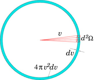
<div style="text-align:center">Figure 9.2: Illustrating the spherical volume in velocity-space over
    which the directional integral is performed.<a id="anglintfig">
</a></div>

<div class="p"><!----></div>
It is necessary to retain just enough information about the anisotropy
of <math xmlns="http://www.w3.org/1998/Math/MathML">
<mrow><mi>f</mi><mo stretchy="false">(</mo><mi mathvariant="bold-italic">v</mi><mo stretchy="false">)</mo></mrow></math> to represent the directed <em>flux density</em> of
neutrons<a 
id="neutron_flux-density92546"></a>, which is what determines their
transport.  Consider neutrons of a specific speed <math xmlns="http://www.w3.org/1998/Math/MathML">
<mrow><mi>v</mi></mrow></math> (i.e.&nbsp;in the
element <math xmlns="http://www.w3.org/1998/Math/MathML">
<mrow><mi mathvariant="italic">dv</mi></mrow></math> at <math xmlns="http://www.w3.org/1998/Math/MathML">
<mrow><mi>v</mi></mrow></math>).  Integrate the full transport equation
(<a href="chap9.xml#neuttrans">9.1</a>) <math xmlns="http://www.w3.org/1998/Math/MathML">
<mrow>
<msup><mrow><mi>v</mi></mrow><mrow><mn>2</mn></mrow>
</msup>

<msup><mrow><mi>d</mi></mrow><mrow><mn>2</mn></mrow>
</msup>
<mi mathvariant="italic">&Omega;</mi></mrow></math> (<math xmlns="http://www.w3.org/1998/Math/MathML">
<mrow><mo>=</mo>
<msup><mrow><mi>d</mi></mrow><mrow><mn>3</mn></mrow>
</msup>
<mi>v</mi><mo stretchy="false">/</mo><mi mathvariant="italic">dv</mi></mrow></math> since <math xmlns="http://www.w3.org/1998/Math/MathML">
<mrow>
<msup><mrow><mi>d</mi></mrow><mrow><mn>3</mn></mrow>
</msup>
<mi>v</mi><mo>=</mo>
<msup><mrow><mi>v</mi></mrow><mrow><mn>2</mn></mrow>
</msup>

<msup><mrow><mi>d</mi></mrow><mrow><mn>2</mn></mrow>
</msup>
<mi mathvariant="italic">&Omega;</mi><mi mathvariant="italic">dv</mi></mrow></math>) over the spherical velocity space element, as illustrated in
Fig.&nbsp;<a href="chap9.xml#anglintfig">9.2</a>. We will denote that
element just <math xmlns="http://www.w3.org/1998/Math/MathML">
<mrow><mi mathvariant="italic">dv</mi></mrow></math>, to remind us of the speed choice, although its
total velocity-space-volume is <math xmlns="http://www.w3.org/1998/Math/MathML">
<mrow><mn>4</mn><mi mathvariant="italic">&pi;</mi>
<msup><mrow><mi>v</mi></mrow><mrow><mn>2</mn></mrow>
</msup>
<mi mathvariant="italic">dv</mi></mrow></math>. Now we denote the
distribution function integrated over direction as
<a id="avergf">
</a><br />
<table width="100%"><tr><td align="center">
    <math xmlns="http://www.w3.org/1998/Math/MathML">
    <mstyle displaystyle="true"><mrow><mi>F</mi><mo stretchy="false">(</mo><mi>v</mi><mo stretchy="false">)</mo><mo>=</mo>
<msub><mrow><mo>&int;</mo></mrow><mrow><mi mathvariant="italic">dv</mi></mrow>
</msub>
<mi>f</mi>
<msup><mrow><mi>v</mi></mrow><mrow><mn>2</mn></mrow>
</msup>

<msup><mrow><mi>d</mi></mrow><mrow><mn>2</mn></mrow>
</msup>
<mi mathvariant="italic">&Omega;</mi><mo>=</mo>
<msub><mrow><mo>&int;</mo></mrow><mrow><mi mathvariant="italic">dv</mi></mrow>
</msub>
<mi>f</mi>
<msup><mrow><mi>d</mi></mrow><mrow><mn>3</mn></mrow>
</msup>
<mi>v</mi><mo stretchy="false">/</mo><mi mathvariant="italic">dv</mi><mo>.</mo></mrow>
    </mstyle></math></td><td width="1">
    <math xmlns="http://www.w3.org/1998/Math/MathML">
    <mstyle displaystyle="true"><mrow><mo stretchy="false">(</mo><mn>9</mn><mo>.</mo><mn>2</mn><mo stretchy="false">)</mo></mrow>
    </mstyle></math>
</td></tr></table>


So the number of particles per unit volume<a 
id="speed-distribution92547"></a>
in the speed range <math xmlns="http://www.w3.org/1998/Math/MathML">
<mrow><mi mathvariant="italic">dv</mi></mrow></math> is <math xmlns="http://www.w3.org/1998/Math/MathML">
<mrow><mi>F</mi><mo stretchy="false">(</mo><mi>v</mi><mo stretchy="false">)</mo><mi mathvariant="italic">dv</mi></mrow></math>. 

<div class="p"><!----></div>
The first term in the
angle-integrated Boltzmann equation becomes <math xmlns="http://www.w3.org/1998/Math/MathML">
<mrow>
<mfrac><mrow><mo>&part;</mo><mi>F</mi></mrow>
<mrow><mo>&part;</mo><mi>t</mi></mrow>
</mfrac>
</mrow></math>.
The second term becomes
<a id="workadvec">
</a><br />
<table width="100%"><tr><td align="center">
    <math xmlns="http://www.w3.org/1998/Math/MathML">
    <mstyle displaystyle="true"><mrow>
<msub><mrow><mo>&int;</mo></mrow><mrow><mi mathvariant="italic">dv</mi></mrow>
</msub>
<mi>v</mi><mi mathvariant="bold-italic">&Omega;</mi><mo>.</mo><mo>&nabla;</mo><mi>f</mi><mi>&ensp;</mi>
<msup><mrow><mi>d</mi></mrow><mrow><mn>3</mn></mrow>
</msup>
<mi>v</mi><mo stretchy="false">/</mo><mi mathvariant="italic">dv</mi><mo>=</mo><mo>&nabla;</mo><mo>.</mo><mo stretchy="false">[</mo>
<msub><mrow><mo>&int;</mo></mrow><mrow><mi mathvariant="italic">dv</mi></mrow>
</msub>
<mi mathvariant="bold-italic">&Omega;</mi><mi mathvariant="italic">vf</mi><mi>&ensp;</mi>
<msup><mrow><mi>d</mi></mrow><mrow><mn>3</mn></mrow>
</msup>
<mi>v</mi><mo stretchy="false">/</mo><mi mathvariant="italic">dv</mi><mo stretchy="false">]</mo><mo>=</mo><mo>&nabla;</mo><mo>.</mo><mi mathvariant="bold-italic">&Gamma;</mi><mo stretchy="false">(</mo><mi>v</mi><mo stretchy="false">)</mo><mo>.</mo></mrow>
    </mstyle></math></td><td width="1">
    <math xmlns="http://www.w3.org/1998/Math/MathML">
    <mstyle displaystyle="true"><mrow><mo stretchy="false">(</mo><mn>9</mn><mo>.</mo><mn>3</mn><mo stretchy="false">)</mo></mrow>
    </mstyle></math>
</td></tr></table>


Here, <math xmlns="http://www.w3.org/1998/Math/MathML">
<mrow><mi mathvariant="bold-italic">&Gamma;</mi><mo stretchy="false">(</mo><mi>v</mi><mo stretchy="false">)</mo><mi mathvariant="italic">dv</mi><mo>=</mo>
<msub><mrow><mo>&int;</mo></mrow><mrow><mi mathvariant="italic">dv</mi></mrow>
</msub>
<mi mathvariant="bold-italic">&Omega;</mi><mi mathvariant="italic">vf</mi><mi>&ensp;</mi>
<msup><mrow><mi>d</mi></mrow><mrow><mn>3</mn></mrow>
</msup>
<mi>v</mi></mrow></math> is the
flux-density of the particles in the speed
element <math xmlns="http://www.w3.org/1998/Math/MathML">
<mrow><mi mathvariant="italic">dv</mi></mrow></math>; so <math xmlns="http://www.w3.org/1998/Math/MathML">
<mrow><mi mathvariant="bold-italic">&Gamma;</mi><mo stretchy="false">(</mo><mi>v</mi><mo stretchy="false">)</mo></mrow></math> is the speed distribution of the
flux-density, a vector quantity.

<div class="p"><!----></div>
Since all <math xmlns="http://www.w3.org/1998/Math/MathML">
<mrow><mi mathvariant="italic">&Sigma;</mi></mrow></math> are independent of <math xmlns="http://www.w3.org/1998/Math/MathML">
<mrow><mi mathvariant="bold-italic">&Omega;</mi></mrow></math> (only the difference
<math xmlns="http://www.w3.org/1998/Math/MathML">
<mrow><mi mathvariant="bold-italic">&Omega;</mi><mo>-</mo><mi mathvariant="bold-italic">&Omega;</mi><mo>'</mo></mrow></math> matters), the first (sink) term on the right of
eq.&nbsp;(<a href="chap9.xml#neuttrans">9.1</a>)
becomes <math xmlns="http://www.w3.org/1998/Math/MathML">
<mrow><mo>-</mo>
<msub><mrow><mi mathvariant="italic">&Sigma;</mi></mrow><mrow><mi>t</mi></mrow>
</msub>
<mi>v</mi><mi>F</mi><mo stretchy="false">(</mo><mi>v</mi><mo stretchy="false">)</mo></mrow></math> and the second (source term) can be written
<a id="neutsource">
</a><br />
<table width="100%"><tr><td align="center">
    <math xmlns="http://www.w3.org/1998/Math/MathML">
    <mstyle displaystyle="true"><mrow><mi>Q</mi><mo stretchy="false">(</mo><mi>v</mi><mo stretchy="false">)</mo><mo>=</mo><mo>&int;</mo><mo stretchy="false">[</mo><mi mathvariant="italic">&nu;</mi>
<msub><mrow><mi mathvariant="italic">&Sigma;</mi></mrow><mrow><mi>f</mi></mrow>
</msub>
<mo stretchy="false">(</mo><mi>v</mi><mo>'</mo><mo>&rarr;</mo><mi>v</mi><mo stretchy="false">)</mo><mo>+</mo>
<msub><mrow><mi mathvariant="italic">&Sigma;</mi></mrow><mrow><mi>s</mi></mrow>
</msub>
<mo stretchy="false">(</mo><mi>v</mi><mo>'</mo><mo>&rarr;</mo><mi>v</mi><mo stretchy="false">)</mo><mo stretchy="false">]</mo><mi>v</mi><mo>'</mo><mi>F</mi><mo stretchy="false">(</mo><mi>v</mi><mo>'</mo><mo stretchy="false">)</mo><mi mathvariant="italic">dv</mi><mo>'</mo><mo>,</mo></mrow>
    </mstyle></math></td><td width="1">
    <math xmlns="http://www.w3.org/1998/Math/MathML">
    <mstyle displaystyle="true"><mrow><mo stretchy="false">(</mo><mn>9</mn><mo>.</mo><mn>4</mn><mo stretchy="false">)</mo></mrow>
    </mstyle></math>
</td></tr></table>


in terms of <math xmlns="http://www.w3.org/1998/Math/MathML">
<mrow>
<msub><mrow><mi mathvariant="italic">&Sigma;</mi></mrow><mrow><mi>f</mi></mrow>
</msub>
</mrow></math> and <math xmlns="http://www.w3.org/1998/Math/MathML">
<mrow>
<msub><mrow><mi mathvariant="italic">&Sigma;</mi></mrow><mrow><mi>s</mi></mrow>
</msub>
</mrow></math> integrated over direction.

<div class="p"><!----></div>
The direction-integrated transport equation is then
<a id="neutspeed">
</a><br />
<table width="100%"><tr><td align="center">
    <math xmlns="http://www.w3.org/1998/Math/MathML">
    <mstyle displaystyle="true"><mrow>
<mfrac><mrow><mo>&part;</mo><mi>F</mi><mo stretchy="false">(</mo><mi>v</mi><mo stretchy="false">)</mo></mrow>
<mrow><mo>&part;</mo><mi>t</mi></mrow>
</mfrac>
<mo>+</mo><mo>&nabla;</mo><mo>.</mo><mi mathvariant="bold-italic">&Gamma;</mi><mo stretchy="false">(</mo><mi>v</mi><mo stretchy="false">)</mo><mo>=</mo><mo>-</mo>
<msub><mrow><mi mathvariant="italic">&Sigma;</mi></mrow><mrow><mi>t</mi></mrow>
</msub>
<mi mathvariant="italic">vF</mi><mo stretchy="false">(</mo><mi>v</mi><mo stretchy="false">)</mo><mo>+</mo><mi>Q</mi><mo stretchy="false">(</mo><mi>v</mi><mo stretchy="false">)</mo><mo>,</mo></mrow>
    </mstyle></math></td><td width="1">
    <math xmlns="http://www.w3.org/1998/Math/MathML">
    <mstyle displaystyle="true"><mrow><mo stretchy="false">(</mo><mn>9</mn><mo>.</mo><mn>5</mn><mo stretchy="false">)</mo></mrow>
    </mstyle></math>
</td></tr></table>


<div class="p"><!----></div>
This equation becomes a diffusion equation if the flux-density is
proportional to the gradient of the density, an approximation usually
called Fick's law<a 
id="Fick_s_law92548"></a>. 
Written in terms of <math xmlns="http://www.w3.org/1998/Math/MathML">
<mrow><mi>F</mi><mo stretchy="false">(</mo><mi>v</mi><mo stretchy="false">)</mo></mrow></math>, this proportionality is
<a id="phifick">
</a><br />
<table width="100%"><tr><td align="center">
    <math xmlns="http://www.w3.org/1998/Math/MathML">
    <mstyle displaystyle="true"><mrow><mi mathvariant="bold-italic">&Gamma;</mi><mo stretchy="false">(</mo><mi>v</mi><mo stretchy="false">)</mo><mo>=</mo><mo>-</mo><mi>D</mi><mo>&nabla;</mo><mi>F</mi><mo stretchy="false">(</mo><mi>v</mi><mo stretchy="false">)</mo><mo>,</mo></mrow>
    </mstyle></math></td><td width="1">
    <math xmlns="http://www.w3.org/1998/Math/MathML">
    <mstyle displaystyle="true"><mrow><mo stretchy="false">(</mo><mn>9</mn><mo>.</mo><mn>6</mn><mo stretchy="false">)</mo></mrow>
    </mstyle></math>
</td></tr></table>


where <math xmlns="http://www.w3.org/1998/Math/MathML">
<mrow><mi>D</mi></mrow></math> is the "diffusion coefficient". The value of <math xmlns="http://www.w3.org/1998/Math/MathML">
<mrow><mi>D</mi></mrow></math>
is approximately <math xmlns="http://www.w3.org/1998/Math/MathML">
<mrow><mi>v</mi><mo stretchy="false">/</mo><mn>3</mn>
<msub><mrow><mi mathvariant="italic">&Sigma;</mi></mrow><mrow><mi>t</mi></mrow>
</msub>
</mrow></math>, as outlined at the end of this
section.
<div class="p"><!----></div>
We then have the speed-resolved (or equivalently
energy-resolved) diffusion 
equation<a 
id="diffusion_equation92549"></a><a 
id="energy_resolved_diffusion92550"></a>
<a id="neutdiff">
</a><br />
<table width="100%"><tr><td align="center">
    <math xmlns="http://www.w3.org/1998/Math/MathML">
    <mstyle displaystyle="true"><mrow>
<mfrac><mrow><mo>&part;</mo><mi>F</mi><mo stretchy="false">(</mo><mi>v</mi><mo stretchy="false">)</mo></mrow>
<mrow><mo>&part;</mo><mi>t</mi></mrow>
</mfrac>
<mo>-</mo><mo>&nabla;</mo><mo>.</mo><mo stretchy="false">[</mo><mi>D</mi><mo>&nabla;</mo><mi>F</mi><mo stretchy="false">(</mo><mi>v</mi><mo stretchy="false">)</mo><mo stretchy="false">]</mo><mo>=</mo><mo>-</mo>
<msub><mrow><mi mathvariant="italic">&Sigma;</mi></mrow><mrow><mi>t</mi></mrow>
</msub>
<mi>v</mi><mi>F</mi><mo stretchy="false">(</mo><mi>v</mi><mo stretchy="false">)</mo><mo>+</mo><mi>Q</mi><mo stretchy="false">(</mo><mi>v</mi><mo stretchy="false">)</mo><mo>.</mo></mrow>
    </mstyle></math></td><td width="1">
    <math xmlns="http://www.w3.org/1998/Math/MathML">
    <mstyle displaystyle="true"><mrow><mo stretchy="false">(</mo><mn>9</mn><mo>.</mo><mn>7</mn><mo stretchy="false">)</mo></mrow>
    </mstyle></math>
</td></tr></table>


The lowest-order anisotropy of <math xmlns="http://www.w3.org/1998/Math/MathML">
<mrow><mi>f</mi><mo stretchy="false">(</mo><mi mathvariant="bold-italic">v</mi><mo stretchy="false">)</mo></mrow></math> is contained in
<math xmlns="http://www.w3.org/1998/Math/MathML">
<mrow><mi mathvariant="bold-italic">&Gamma;</mi><mo>=</mo><mi>D</mi><mo>&nabla;</mo><mi>F</mi><mo stretchy="false">(</mo><mi>v</mi><mo stretchy="false">)</mo></mrow></math>, but the collision terms in this approximation are
independent of any anisotropy. The equation applies for all values of
the speed, <math xmlns="http://www.w3.org/1998/Math/MathML">
<mrow><mi>v</mi></mrow></math>.

<div class="p"><!----></div>
<br /><br />
<span class="footnotesize">
<b>Enrichment: Derivation of Diffusion Coefficient.</b>

<div class="p"><!----></div>
  The neutron (kinetic)
  transport equation (<a href="chap9.xml#neuttrans">9.1</a>) can be turned into a spatial
  diffusion equation by considering a fixed speed <math xmlns="http://www.w3.org/1998/Math/MathML">
<mrow><mi>v</mi></mrow></math>.  To lowest
  order, we approximate the angular dependence of <math xmlns="http://www.w3.org/1998/Math/MathML">
<mrow><mi>f</mi></mrow></math> as
  being a constant plus a term proportional to <math xmlns="http://www.w3.org/1998/Math/MathML">
<mrow><mi mathvariant="italic">&mu;</mi><mo>=</mo><mi>cos</mi><mi mathvariant="italic">&theta;</mi></mrow></math>; i.e.&nbsp;  as <math xmlns="http://www.w3.org/1998/Math/MathML">
<mrow><mi>f</mi><mo>=</mo>
<msub><mrow><mi>f</mi></mrow><mrow><mn>0</mn></mrow>
</msub>
<mo>+</mo>
<msub><mrow><mi>f</mi></mrow><mrow><mn>1</mn></mrow>
</msub>
<mi mathvariant="italic">&mu;</mi></mrow></math>, where <math xmlns="http://www.w3.org/1998/Math/MathML">
<mrow>
<msub><mrow><mi>f</mi></mrow><mrow><mn>0</mn></mrow>
</msub>
</mrow></math> and <math xmlns="http://www.w3.org/1998/Math/MathML">
<mrow>
<msub><mrow><mi>f</mi></mrow><mrow><mn>1</mn></mrow>
</msub>
</mrow></math> are independent of
  <math xmlns="http://www.w3.org/1998/Math/MathML">
<mrow><mi mathvariant="bold-italic">&Omega;</mi></mrow></math>. These are the first two terms of an expansion of the
  angular dependence in spherical harmonics. Reactor physics
  literature calls this the <math xmlns="http://www.w3.org/1998/Math/MathML">
<mrow>
<msub><mrow><mi>P</mi></mrow><mrow><mn>1</mn></mrow>
</msub>
</mrow></math> Approximation.  Obviously this
  approximation only makes sense if the distribution has an
  approximate axis of (velocity) cylindrical symmetry, relative to
  which the polar angle <math xmlns="http://www.w3.org/1998/Math/MathML">
<mrow><mi mathvariant="italic">&theta;</mi></mrow></math> is measured.  In the absence of
  inherent material anisotropy, the local axis of symmetry must be in
  the direction of of the density gradient <math xmlns="http://www.w3.org/1998/Math/MathML">
<mrow><mo>&nabla;</mo>
<msub><mrow><mi>f</mi></mrow><mrow><mn>0</mn></mrow>
</msub>
</mrow></math>.

<div class="p"><!----></div>
  &nbsp;&nbsp;&nbsp;&nbsp;&nbsp;&nbsp;
    <br /><table border="0" align="left"><tr><td></td><td width="500">

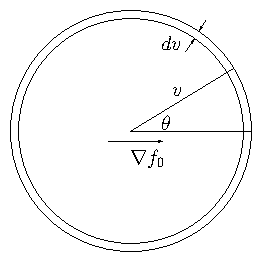
      Integration over a spherical velocity element with
      <math xmlns="http://www.w3.org/1998/Math/MathML">
<mrow><mi mathvariant="italic">&mu;</mi><mo>=</mo><mi>cos</mi><mi mathvariant="italic">&theta;</mi></mrow></math> and the angle <math xmlns="http://www.w3.org/1998/Math/MathML">
<mrow><mi mathvariant="italic">&theta;</mi></mrow></math> measured from the
      direction <math xmlns="http://www.w3.org/1998/Math/MathML">
<mrow><mo>&nabla;</mo>
<msub><mrow><mi>f</mi></mrow><mrow><mn>0</mn></mrow>
</msub>
</mrow></math>.<br /> 
</td></tr></table><!--vbox-->&nbsp;&nbsp;&nbsp;
    <img src="figures/costhetasphere2.png" alt="figures/costhetasphere2.png" />
  <!--hbox--><br clear="all" />

<div class="p"><!----></div>
  If we substitute into eq.&nbsp;  (<a href="chap9.xml#neuttrans">9.1</a>) and equate orders of <math xmlns="http://www.w3.org/1998/Math/MathML">
<mrow><mi mathvariant="italic">&mu;</mi></mrow></math>, ignoring the partial
  time derivative (since we presume the distribution in angle relaxes
  quickly), we then obtain at order <math xmlns="http://www.w3.org/1998/Math/MathML">
<mrow><mi mathvariant="italic">&mu;</mi></mrow></math>
  <br />
<table width="100%"><tr><td align="center">
    <math xmlns="http://www.w3.org/1998/Math/MathML">
    <mstyle displaystyle="true"><mrow><mo stretchy="false">&verbar;</mo><mo>&nabla;</mo>
<msub><mrow><mi>f</mi></mrow><mrow><mn>0</mn></mrow>
</msub>
<mo stretchy="false">&verbar;</mo><mo>=</mo><mo stretchy="false">(</mo><mo>-</mo>
<msub><mrow><mi mathvariant="italic">&Sigma;</mi></mrow><mrow><mi>t</mi></mrow>
</msub>
<mo>+</mo>
<msub><mrow><mi mathvariant="italic">&Sigma;</mi></mrow><mrow><mi>s</mi><mn>1</mn></mrow>
</msub>
<mo stretchy="false">)</mo>
<msub><mrow><mi>f</mi></mrow><mrow><mn>1</mn></mrow>
</msub>
<mo>,</mo></mrow>
    </mstyle></math>
</td></tr></table>
<br />

  where <math xmlns="http://www.w3.org/1998/Math/MathML">
<mrow>
<msub><mrow><mi mathvariant="italic">&Sigma;</mi></mrow><mrow><mi>s</mi><mn>1</mn></mrow>
</msub>
</mrow></math> is the part of the scattering term proportional
  to <math xmlns="http://www.w3.org/1998/Math/MathML">
<mrow><mi mathvariant="italic">&mu;</mi></mrow></math>, which is always smaller than <math xmlns="http://www.w3.org/1998/Math/MathML">
<mrow>
<msub><mrow><mi mathvariant="italic">&Sigma;</mi></mrow><mrow><mi>t</mi></mrow>
</msub>
</mrow></math>. (Sometimes
  <math xmlns="http://www.w3.org/1998/Math/MathML">
<mrow>
<msub><mrow><mi mathvariant="italic">&Sigma;</mi></mrow><mrow><mi>s</mi><mn>1</mn></mrow>
</msub>
</mrow></math> is approximately ignorable.) Unlike scattering,
  fission does not contribute to this anisotropic component, except
  from its part in <math xmlns="http://www.w3.org/1998/Math/MathML">
<mrow>
<msub><mrow><mi mathvariant="italic">&Sigma;</mi></mrow><mrow><mi>t</mi></mrow>
</msub>
</mrow></math>, because it is generally presumed that
  there is no significant correlation between the direction of neutron
  emission from a fission event and the incoming neutron. [The degree
  of anisotropy in neutrons from fission reactions is low but
  formally non-zero, especially at higher incoming neutron energy.]

<div class="p"><!----></div>
  The contribution from
  the speed element <math xmlns="http://www.w3.org/1998/Math/MathML">
<mrow><mi mathvariant="italic">dv</mi></mrow></math> to the directed
  spatial flux density (which is along the symmetry axis direction) is
  <br />
<table width="100%"><tr><td align="center">
    <math xmlns="http://www.w3.org/1998/Math/MathML">
    <mstyle displaystyle="true"><mrow><mi mathvariant="italic">&Gamma;</mi><mo stretchy="false">(</mo><mi>v</mi><mo stretchy="false">)</mo><mi mathvariant="italic">dv</mi><mo>=</mo><mo>&int;</mo><mi>f</mi><mi>v</mi><mi mathvariant="italic">&mu;</mi>
<msup><mrow><mi>d</mi></mrow><mrow><mn>3</mn></mrow>
</msup>
<mi>v</mi><mo>=</mo><mo>&int;</mo><mi mathvariant="italic">fv</mi><mi mathvariant="italic">&mu;</mi><mi>&ensp;</mi><mn>2</mn><mi mathvariant="italic">&pi;</mi>
<msup><mrow><mi>v</mi></mrow><mrow><mn>2</mn></mrow>
</msup>
<mi>d</mi><mi mathvariant="italic">&mu;</mi><mi mathvariant="italic">dv</mi><mo>=</mo><mn>2</mn><mi mathvariant="italic">&pi;</mi>
<msup><mrow><mi>v</mi></mrow><mrow><mn>3</mn></mrow>
</msup>
<mi mathvariant="italic">dv</mi><mo>&int;</mo><mo stretchy="false">(</mo>
<msub><mrow><mi>f</mi></mrow><mrow><mn>0</mn></mrow>
</msub>
<mo>+</mo>
<msub><mrow><mi>f</mi></mrow><mrow><mn>1</mn></mrow>
</msub>
<mi mathvariant="italic">&mu;</mi><mo stretchy="false">)</mo><mi mathvariant="italic">&mu;</mi><mi>d</mi><mi mathvariant="italic">&mu;</mi><mo>=</mo>
<mfrac><mrow><mn>1</mn></mrow>
<mrow><mn>3</mn></mrow>
</mfrac>

<msub><mrow><mi mathvariant="italic">vf</mi></mrow><mrow><mn>1</mn></mrow>
</msub>
<mi>&ensp;</mi><mn>4</mn><mi mathvariant="italic">&pi;</mi>
<msup><mrow><mi>v</mi></mrow><mrow><mn>2</mn></mrow>
</msup>
<mi mathvariant="italic">dv</mi><mo>.</mo></mrow>
    </mstyle></math>
</td></tr></table>
<br />

  Incorporating the previous equation, we then have
  <br />
<table width="100%"><tr><td align="center">
    <math xmlns="http://www.w3.org/1998/Math/MathML">
    <mstyle displaystyle="true"><mrow><mi mathvariant="bold-italic">&Gamma;</mi><mo stretchy="false">(</mo><mi>v</mi><mo stretchy="false">)</mo><mo>=</mo><mo>-</mo>
<mfrac><mrow><mi>v</mi></mrow>
<mrow><mn>3</mn><mo stretchy="false">(</mo>
<msub><mrow><mi mathvariant="italic">&Sigma;</mi></mrow><mrow><mi>t</mi></mrow>
</msub>
<mo>-</mo>
<msub><mrow><mi mathvariant="italic">&Sigma;</mi></mrow><mrow><mi>s</mi><mn>1</mn></mrow>
</msub>
<mo stretchy="false">)</mo></mrow>
</mfrac>
<mo>&nabla;</mo><mo stretchy="false">(</mo>
<msub><mrow><mi>f</mi></mrow><mrow><mn>0</mn></mrow>
</msub>
<mn>4</mn><mi mathvariant="italic">&pi;</mi>
<msup><mrow><mi>v</mi></mrow><mrow><mn>2</mn></mrow>
</msup>
<mo stretchy="false">)</mo><mo>.</mo></mrow>
    </mstyle></math>
</td></tr></table>
<br />

  This is Fick's law relating a flux density <math xmlns="http://www.w3.org/1998/Math/MathML">
<mrow><mi mathvariant="bold-italic">&Gamma;</mi><mi mathvariant="italic">dv</mi></mrow></math> to the
  gradient of a density <math xmlns="http://www.w3.org/1998/Math/MathML">
<mrow><mi>f</mi><mn>4</mn><mi mathvariant="italic">&pi;</mi>
<msup><mrow><mi>v</mi></mrow><mrow><mn>2</mn></mrow>
</msup>
<mi mathvariant="italic">dv</mi></mrow></math>, times a diffusivity 
  <br />
<table width="100%"><tr><td align="center">
    <math xmlns="http://www.w3.org/1998/Math/MathML">
    <mstyle displaystyle="true"><mrow><mi>D</mi><mo>=</mo>
<mfrac><mrow><mi>v</mi></mrow>
<mrow><mn>3</mn><mo stretchy="false">(</mo>
<msub><mrow><mi mathvariant="italic">&Sigma;</mi></mrow><mrow><mi>t</mi></mrow>
</msub>
<mo>-</mo>
<msub><mrow><mi mathvariant="italic">&Sigma;</mi></mrow><mrow><mi>s</mi><mn>1</mn></mrow>
</msub>
<mo stretchy="false">)</mo></mrow>
</mfrac>
<mo>.</mo></mrow>
    </mstyle></math>
</td></tr></table>
<br />

</span>

<div class="p"><!----></div>
 <a id="tth_sEc9.3"></a><h2>
9.3&nbsp;&nbsp;Numerical Representation of Multigroup Equations</h2>

<div class="p"><!----></div>
We've made substantial progress in making the transport equation more
managable, lowering its dimensionality from six phase-space dimensions
to four (3 space and 1 speed). Even so, we have to choose how to
represent the distribution in speed (or energy), as well as the
spatial representation.

<div class="p"><!----></div>
     <a id="tth_sEc9.3.1"></a><h3>
9.3.1&nbsp;&nbsp;Groups</h3>

<div class="p"><!----></div>
<a 
id="groups93551"></a><a 
id="speed_groups93552"></a>
<div class="p"><!----></div>
<a id="tth_fIg9.3">
</a>   <img src="figures/speedgroups.png" alt="figures/speedgroups.png" /><a id="speedgroups">
</a>
  
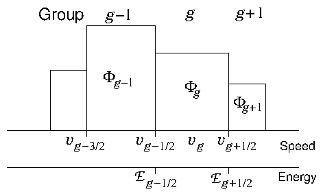
<div style="text-align:center">Figure 9.3: Groups are ranges in speed (equivalently energy) into which
    the neutrons are lumped. They are very rarely of equal width in
    speed or energy.<a id="speedgroupsl">
</a></div>

<div class="p"><!----></div>
The natural discretization in speed is to use ranges of speed, or
equivalently energy.
In reactor physics the ranges are called "groups". It is like
representing the speed distribution as a histogram (see Fig.&nbsp;<a href="chap9.xml#speedgroupsl">9.3</a>). A point in phase
space (particle, if you like) belongs to the (integer) group <math xmlns="http://www.w3.org/1998/Math/MathML">
<mrow><mi>g</mi></mrow></math> if
its speed satisfies <math xmlns="http://www.w3.org/1998/Math/MathML">
<mrow>
<msub><mrow><mi>v</mi></mrow><mrow><mi>g</mi><mo>-</mo><mn>1</mn><mo stretchy="false">/</mo><mn>2</mn></mrow>
</msub>
<mo>&le;</mo><mi>v</mi><mo>&lt;</mo>
<msub><mrow><mi>v</mi></mrow><mrow><mi>g</mi><mo>+</mo><mn>1</mn><mo stretchy="false">/</mo><mn>2</mn></mrow>
</msub>
</mrow></math>. The
half-integer-index speeds are the extrema of the speed range belonging
to group <math xmlns="http://www.w3.org/1998/Math/MathML">
<mrow><mi>g</mi></mrow></math>, and this group is regarded as having a typical or
average speed <math xmlns="http://www.w3.org/1998/Math/MathML">
<mrow>
<msub><mrow><mi>v</mi></mrow><mrow><mi>g</mi></mrow>
</msub>
</mrow></math>. Put another way, the group can be considered to
be the integral over the finite speed element <math xmlns="http://www.w3.org/1998/Math/MathML">
<mrow><mi mathvariant="italic">&Delta;</mi>
<msub><mrow><mi>v</mi></mrow><mrow><mi>g</mi></mrow>
</msub>
<mo>=</mo>
<msub><mrow><mi>v</mi></mrow><mrow><mi>g</mi><mo>+</mo><mn>1</mn><mo stretchy="false">/</mo><mn>2</mn></mrow>
</msub>
<mo>-</mo>
<msub><mrow><mi>v</mi></mrow><mrow><mi>g</mi><mo>-</mo><mn>1</mn><mo stretchy="false">/</mo><mn>2</mn></mrow>
</msub>
</mrow></math>. Take there to be <math xmlns="http://www.w3.org/1998/Math/MathML">
<mrow>
<msub><mrow><mi>N</mi></mrow><mrow><mi>G</mi></mrow>
</msub>
</mrow></math> groups in all.
Then each neutron group separately satisfies a diffusion equation like
(<a href="chap9.xml#neutdiff">9.7</a>), except that the source integral <math xmlns="http://www.w3.org/1998/Math/MathML">
<mrow><mi>Q</mi><mo stretchy="false">(</mo><mi>v</mi><mo stretchy="false">)</mo></mrow></math> for each
group contains, in its integral, contributions from all the other
groups, corresponding to fission neutrons appearing in one group when
they were caused by another group, or scattering directly from one
speed (group) to another. 
<a id="multigroupdiff">
</a><br />
<table width="100%"><tr><td align="center">
    <math xmlns="http://www.w3.org/1998/Math/MathML">
    <mstyle displaystyle="true"><mrow>
<mfrac><mrow><mo>&part;</mo>
<msub><mrow><mi>F</mi></mrow><mrow><mi>g</mi></mrow>
</msub>
</mrow>
<mrow><mo>&part;</mo><mi>t</mi></mrow>
</mfrac>
<mo>-</mo><mo>&nabla;</mo><mo>.</mo><mo stretchy="false">[</mo>
<msub><mrow><mi>D</mi></mrow><mrow><mi>g</mi></mrow>
</msub>
<mo>&nabla;</mo>
<msub><mrow><mi>F</mi></mrow><mrow><mi>g</mi></mrow>
</msub>
<mo stretchy="false">]</mo><mo>+</mo>
<msub><mrow><mi mathvariant="italic">&Sigma;</mi></mrow><mrow><mi mathvariant="italic">tg</mi></mrow>
</msub>

<msub><mrow><mi>v</mi></mrow><mrow><mi>g</mi></mrow>
</msub>

<msub><mrow><mi>F</mi></mrow><mrow><mi>g</mi></mrow>
</msub>
<mo>=</mo>
<msub><mrow><mi>Q</mi></mrow><mrow><mi>g</mi></mrow>
</msub>
<mo>.</mo></mrow>
    </mstyle></math></td><td width="1">
    <math xmlns="http://www.w3.org/1998/Math/MathML">
    <mstyle displaystyle="true"><mrow><mo stretchy="false">(</mo><mn>9</mn><mo>.</mo><mn>8</mn><mo stretchy="false">)</mo></mrow>
    </mstyle></math>
</td></tr></table>


Since <math xmlns="http://www.w3.org/1998/Math/MathML">
<mrow><mi>Q</mi></mrow></math> depends linearly on the <math xmlns="http://www.w3.org/1998/Math/MathML">
<mrow>
<msub><mrow><mi>F</mi></mrow><mrow><mi>g</mi></mrow>
</msub>
</mrow></math>, through the integrals
<math xmlns="http://www.w3.org/1998/Math/MathML">
<mrow><mo>&int;</mo><mi>v</mi><mo>'</mo><mi>F</mi><mo stretchy="false">(</mo><mi>v</mi><mo>'</mo><mo stretchy="false">)</mo><mi mathvariant="italic">dv</mi><mo>'</mo></mrow></math>, the discretized equations
are naturally expressed in terms of a matrix equation acting on a column
vector of group fluxes
<a id="multigroupdiffvec">
</a><br />
<table width="100%"><tr><td align="center">
    <math xmlns="http://www.w3.org/1998/Math/MathML">
    <mstyle displaystyle="true"><mrow>
<mfrac><mrow><mo>&part;</mo><mi mathvariant="bold">F</mi></mrow>
<mrow><mo>&part;</mo><mi>t</mi></mrow>
</mfrac>
<mo>+</mo><mo stretchy="false">(</mo><mo>-</mo><mi mathvariant="bold">L</mi><mo>+</mo>
<msub><mrow><mi mathvariant="bold-italic">&Sigma;</mi></mrow><mrow><mi>t</mi></mrow>
</msub>
<mi mathvariant="bold">V</mi><mo stretchy="false">)</mo><mi mathvariant="bold">F</mi><mo>=</mo><mi mathvariant="bold">Q</mi><mo>=</mo><mi mathvariant="bold">A</mi><mi mathvariant="bold">F</mi><mo>.</mo></mrow>
    </mstyle></math></td><td width="1">
    <math xmlns="http://www.w3.org/1998/Math/MathML">
    <mstyle displaystyle="true"><mrow><mo stretchy="false">(</mo><mn>9</mn><mo>.</mo><mn>9</mn><mo stretchy="false">)</mo></mrow>
    </mstyle></math>
</td></tr></table>


The <math xmlns="http://www.w3.org/1998/Math/MathML">
<mrow>
<msub><mrow><mi>N</mi></mrow><mrow><mi>G</mi></mrow>
</msub>
<mo>&times;</mo>
<msub><mrow><mi>N</mi></mrow><mrow><mi>G</mi></mrow>
</msub>
</mrow></math> matrices <math xmlns="http://www.w3.org/1998/Math/MathML">
<mrow><mi mathvariant="bold">L</mi></mrow></math>, <math xmlns="http://www.w3.org/1998/Math/MathML">
<mrow>
<msub><mrow><mi mathvariant="bold-italic">&Sigma;</mi></mrow><mrow><mi>t</mi></mrow>
</msub>
</mrow></math> and <math xmlns="http://www.w3.org/1998/Math/MathML">
<mrow><mi mathvariant="bold">V</mi></mrow></math> are
diagonal<a 
id="matrix_diagonal93553"></a>, and their <math xmlns="http://www.w3.org/1998/Math/MathML">
<mrow><mi>g</mi></mrow></math>th diagonal elements are <math xmlns="http://www.w3.org/1998/Math/MathML">
<mrow><mo>&nabla;</mo><mo>.</mo>
<msub><mrow><mi>D</mi></mrow><mrow><mi>g</mi></mrow>
</msub>
<mo>&nabla;</mo></mrow></math>,
<math xmlns="http://www.w3.org/1998/Math/MathML">
<mrow>
<msub><mrow><mi mathvariant="italic">&Sigma;</mi></mrow><mrow><mi mathvariant="italic">tg</mi></mrow>
</msub>
</mrow></math>, and <math xmlns="http://www.w3.org/1998/Math/MathML">
<mrow>
<msub><mrow><mi>v</mi></mrow><mrow><mi>g</mi></mrow>
</msub>
</mrow></math>, respectively. Matrix <math xmlns="http://www.w3.org/1998/Math/MathML">
<mrow><mi mathvariant="bold">A</mi></mrow></math>, which
multiplies <math xmlns="http://www.w3.org/1998/Math/MathML">
<mrow><mi mathvariant="bold">F</mi></mrow></math> to provide the source term <math xmlns="http://www.w3.org/1998/Math/MathML">
<mrow><mi mathvariant="bold">Q</mi></mrow></math>, is not
diagonal. It couples together the different rows of the matrix
equation, the different groups. The crucial point is that the
collision matrices <math xmlns="http://www.w3.org/1998/Math/MathML">
<mrow>
<msub><mrow><mi mathvariant="bold-italic">&Sigma;</mi></mrow><mrow><mi>t</mi></mrow>
</msub>
</mrow></math> and <math xmlns="http://www.w3.org/1998/Math/MathML">
<mrow><mi mathvariant="bold">A</mi></mrow></math> can be calculated at any
position <math xmlns="http://www.w3.org/1998/Math/MathML">
<mrow><mi mathvariant="bold-italic">x</mi></mrow></math> by performing appropriate integrals over speed <math xmlns="http://www.w3.org/1998/Math/MathML">
<mrow><mi>v</mi></mrow></math>
and then sums over different nuclear species. These require extensive
information about the cross-sections for different types of
collisions, but the velocity integrals only have to be done once.

<div class="p"><!----></div>

<b>Spatially Uniform Problem&nbsp;&nbsp;</b> If we are treating an idealized
"infinite homogeneous" reactor, then all the coefficients of the
"leakage operator"<a 
id="leakage_operator93554"></a> <math xmlns="http://www.w3.org/1998/Math/MathML">
<mrow><mi mathvariant="bold">L</mi></mrow></math> are zero:
<math xmlns="http://www.w3.org/1998/Math/MathML">
<mrow><mo>&nabla;</mo><mo>.</mo>
<msub><mrow><mi>D</mi></mrow><mrow><mi>g</mi></mrow>
</msub>
<mo>&nabla;</mo><mo>=</mo><mn>0</mn></mrow></math>. The spatial derivative terms are
negligible. We need not represent more than one position in space, so
the multiple group fluxes represent the only different dependent
variable components we need to solve for. We have a first order
ordinary differential vector equation with time as the only
independent variable<a href="footnote.xml#tthFtNtAFB" id="tthFrefAFB"><math xmlns="http://www.w3.org/1998/Math/MathML">
<mrow>
<msup><mrow></mrow><mrow><mn>51</mn></mrow>
</msup>
</mrow></math></a>.  In such a situation one might use a large
number of speed groups <math xmlns="http://www.w3.org/1998/Math/MathML">
<mrow>
<msub><mrow><mi>N</mi></mrow><mrow><mi>G</mi></mrow>
</msub>
</mrow></math>. The system can be solved by the methods
of chapter <a href="chap2.xml#ODEChap">2</a>.

<div class="p"><!----></div>

<b>Non-uniform Problem&nbsp;&nbsp;</b> In an inhomogeneous or finite sized
reactor<a 
id="nuclear_reactor93555"></a>, the diffusive
transport<a 
id="diffusion93556"></a> terms cannot be ignored. In principle, we
can then discretize the reactor in space, producing a total of (say)
<math xmlns="http://www.w3.org/1998/Math/MathML">
<mrow>
<msub><mrow><mi>N</mi></mrow><mrow><mi>S</mi></mrow>
</msub>
</mrow></math> elements. Of course for a stuctured two dimensional mesh
<math xmlns="http://www.w3.org/1998/Math/MathML">
<mrow>
<msub><mrow><mi>N</mi></mrow><mrow><mi>S</mi></mrow>
</msub>
<mo>=</mo>
<msub><mrow><mi>N</mi></mrow><mrow><mn>1</mn></mrow>
</msub>
<mo>&times;</mo>
<msub><mrow><mi>N</mi></mrow><mrow><mn>2</mn></mrow>
</msub>
</mrow></math> or three dimensional <math xmlns="http://www.w3.org/1998/Math/MathML">
<mrow>
<msub><mrow><mi>N</mi></mrow><mrow><mi>S</mi></mrow>
</msub>
<mo>=</mo>
<msub><mrow><mi>N</mi></mrow><mrow><mn>1</mn></mrow>
</msub>
<mo>&times;</mo>
<msub><mrow><mi>N</mi></mrow><mrow><mn>2</mn></mrow>
</msub>
<mo>&times;</mo>
<msub><mrow><mi>N</mi></mrow><mrow><mn>3</mn></mrow>
</msub>
</mrow></math>. At each of the <math xmlns="http://www.w3.org/1998/Math/MathML">
<mrow>
<msub><mrow><mi>N</mi></mrow><mrow><mi>S</mi></mrow>
</msub>
</mrow></math> spatial elements there are <math xmlns="http://www.w3.org/1998/Math/MathML">
<mrow>
<msub><mrow><mi>N</mi></mrow><mrow><mi>G</mi></mrow>
</msub>
</mrow></math> groups,
each of which has a speed-distribution component <math xmlns="http://www.w3.org/1998/Math/MathML">
<mrow>
<msub><mrow><mi>F</mi></mrow><mrow><mi>g</mi></mrow>
</msub>
</mrow></math>. So there are a
total of <math xmlns="http://www.w3.org/1998/Math/MathML">
<mrow>
<msub><mrow><mi>N</mi></mrow><mrow><mi>S</mi></mrow>
</msub>
<mo>&times;</mo>
<msub><mrow><mi>N</mi></mrow><mrow><mi>G</mi></mrow>
</msub>
</mrow></math> <math xmlns="http://www.w3.org/1998/Math/MathML">
<mrow>
<msub><mrow><mi>F</mi></mrow><mrow><mi>g</mi></mrow>
</msub>
<mo stretchy="false">(</mo><mi mathvariant="bold-italic">x</mi><mo stretchy="false">)</mo></mrow></math>-values to solve
for<a href="footnote.xml#tthFtNtAFC" id="tthFrefAFC"><math xmlns="http://www.w3.org/1998/Math/MathML">
<mrow>
<msup><mrow></mrow><mrow><mn>52</mn></mrow>
</msup>
</mrow></math></a>. In
principle, we can line all these values up into a single column
vector, then we can express the diffusion term (<math xmlns="http://www.w3.org/1998/Math/MathML">
<mrow><mi mathvariant="bold">L</mi><mi mathvariant="bold">F</mi></mrow></math>) as
finite differences between components adjacent in space. So it becomes
a true multiplicative matrix rather than a matrix of differential
operators.

<div class="p"><!----></div>
We can in principle then advance the diffusion equation in time using
an explicit scheme. In this situation the stability of our numerical
scheme depends upon the diffusive nature of the <math xmlns="http://www.w3.org/1998/Math/MathML">
<mrow><mi>D</mi></mrow></math> term. We need to
recall the considerations for parabolic diffusion equations from
Chapter <a href="chap5.xml#DiffusionChap">5</a>.  An explicit FTCS scheme, requires us to
satisfy the stability condition <math xmlns="http://www.w3.org/1998/Math/MathML">
<mrow><mi mathvariant="italic">&Delta;</mi><mi>t</mi><mo>&le;</mo><mi mathvariant="italic">&Delta;</mi>
<msup><mrow><mi>x</mi></mrow><mrow><mn>2</mn></mrow>
</msup>
<mo stretchy="false">/</mo><mn>2</mn>
<msub><mrow><mi>N</mi></mrow><mrow><mi>d</mi></mrow>
</msub>
<mi>D</mi></mrow></math>
where <math xmlns="http://www.w3.org/1998/Math/MathML">
<mrow>
<msub><mrow><mi>N</mi></mrow><mrow><mi>d</mi></mrow>
</msub>
</mrow></math> is the number of space dimensions. Now <math xmlns="http://www.w3.org/1998/Math/MathML">
<mrow><mi>D</mi><mo>&ap;</mo>
<mfrac><mrow><mn>1</mn></mrow>
<mrow><mn>3</mn></mrow>
</mfrac>
<mi>v</mi>
<msub><mrow><mi mathvariant="italic">&ell;</mi></mrow><mrow><mi>c</mi></mrow>
</msub>
</mrow></math>, where <math xmlns="http://www.w3.org/1998/Math/MathML">
<mrow>
<msub><mrow><mi mathvariant="italic">&ell;</mi></mrow><mrow><mi>c</mi></mrow>
</msub>
</mrow></math> is the collision
mean-free-path. Consequently the stability condition can be considered
to be
<a id="neutdiffstab">
</a><br />
<table width="100%"><tr><td align="center">
    <math xmlns="http://www.w3.org/1998/Math/MathML">
    <mstyle displaystyle="true"><mrow><mi mathvariant="italic">&Delta;</mi><mi mathvariant="italic">&ell;</mi><mo>&equiv;</mo><mi>v</mi><mi mathvariant="italic">&Delta;</mi><mi>t</mi><mo>&le;</mo>
<mfrac><mrow><mn>3</mn></mrow>
<mrow><mn>2</mn>
<msub><mrow><mi>N</mi></mrow><mrow><mi>d</mi></mrow>
</msub>
</mrow>
</mfrac>

<mfrac><mrow><mi mathvariant="italic">&Delta;</mi><mi>x</mi></mrow>
<mrow>
<msub><mrow><mi mathvariant="italic">&ell;</mi></mrow><mrow><mi>c</mi></mrow>
</msub>
</mrow>
</mfrac>
<mi mathvariant="italic">&Delta;</mi><mi>x</mi><mo>.</mo></mrow>
    </mstyle></math></td><td width="1">
    <math xmlns="http://www.w3.org/1998/Math/MathML">
    <mstyle displaystyle="true"><mrow><mo stretchy="false">(</mo><mn>9</mn><mo>.</mo><mn>10</mn><mo stretchy="false">)</mo></mrow>
    </mstyle></math>
</td></tr></table>


The distance a neutron travels during the timestep must be less than
<math xmlns="http://www.w3.org/1998/Math/MathML">
<mrow><mi mathvariant="italic">&Delta;</mi><mi>x</mi></mrow></math> times a factor <math xmlns="http://www.w3.org/1998/Math/MathML">
<mrow><mn>3</mn><mi mathvariant="italic">&Delta;</mi><mi>x</mi><mo stretchy="false">/</mo><mn>2</mn>
<msub><mrow><mi>N</mi></mrow><mrow><mi>d</mi></mrow>
</msub>

<msub><mrow><mi mathvariant="italic">&ell;</mi></mrow><mrow><mi>c</mi></mrow>
</msub>
</mrow></math>, for stability.
Superthermal neutrons are liable to be the most limiting of <math xmlns="http://www.w3.org/1998/Math/MathML">
<mrow><mi mathvariant="italic">&Delta;</mi><mi>t</mi></mrow></math>, because their speed <math xmlns="http://www.w3.org/1998/Math/MathML">
<mrow><mi>v</mi></mrow></math> is greater (higher energy), and their
<math xmlns="http://www.w3.org/1998/Math/MathML">
<mrow>
<msub><mrow><mi mathvariant="italic">&ell;</mi></mrow><mrow><mi>c</mi></mrow>
</msub>
</mrow></math> is longer (smaller collision cross-section).

<div class="p"><!----></div>
     <a id="tth_sEc9.3.2"></a><h3>
9.3.2&nbsp;&nbsp;Steady State Eigenvalue</h3>

<div class="p"><!----></div>
The most significant aspect of the neutron diffusion equation, as
applied to a fission reactor, is that it is a homogeneous
equation<a href="footnote.xml#tthFtNtAFD" id="tthFrefAFD"><math xmlns="http://www.w3.org/1998/Math/MathML">
<mrow>
<msup><mrow></mrow><mrow><mn>53</mn></mrow>
</msup>
</mrow></math></a>,
meaning that every term in eq.&nbsp;(<a href="chap9.xml#multigroupdiffvec">9.9</a>) is
proportional to <math xmlns="http://www.w3.org/1998/Math/MathML">
<mrow><mi mathvariant="bold">F</mi></mrow></math>. That is because in a reactor essentially all
the neutrons are generated by the fission reactions caused by the
neutron flux itself.  The steady state solution of a homogeneous equation is
identically zero unless the multiplying matrix happens to be
singular; in other words unless its determinant is zero. So the
condition for there to be a non-trivial steady solution, representing
a steadily operating reactor, to the multigroup diffusion equations
is:
<a id="mgsteady">
</a><br />
<table width="100%"><tr><td align="center">
    <math xmlns="http://www.w3.org/1998/Math/MathML">
    <mstyle displaystyle="true"><mrow><mo>det</mo><mo stretchy="false">(</mo><mi mathvariant="bold">L</mi><mo>-</mo><mi mathvariant="bold-italic">&Sigma;</mi><mi mathvariant="bold">V</mi><mo>+</mo><mi mathvariant="bold">A</mi><mo stretchy="false">)</mo><mo>=</mo><mn>0</mn><mo>.</mo></mrow>
    </mstyle></math></td><td width="1">
    <math xmlns="http://www.w3.org/1998/Math/MathML">
    <mstyle displaystyle="true"><mrow><mo stretchy="false">(</mo><mn>9</mn><mo>.</mo><mn>11</mn><mo stretchy="false">)</mo></mrow>
    </mstyle></math>
</td></tr></table>


Such a condition does not come about by luck. It must be carefully
arranged by adjusting the reactivity of the reactor using control
rods<a 
id="control_rod93557"></a>
and so on. If this condition of "criticality"<a 
id="criticality93558"></a> is
not satisfied, then the solution is <em>not steady</em>, the power is
either increasing or decreasing with time. The way the condition is
generally represented in the mathematics is by the idealized
supposition that one has a way to adjust the effective neutron yield
of all fission reactions; in particular, that they can be multiplied
by a reactivity factor <math xmlns="http://www.w3.org/1998/Math/MathML">
<mrow><mn>1</mn><mo stretchy="false">/</mo><mi>k</mi></mrow></math>. Remember that <math xmlns="http://www.w3.org/1998/Math/MathML">
<mrow><mi>Q</mi><mo stretchy="false">(</mo><mi>v</mi><mo stretchy="false">)</mo></mrow></math> arose from two
terms: scattering and fission. Write them separately as
<math xmlns="http://www.w3.org/1998/Math/MathML">
<mrow>
<msub><mrow><mi mathvariant="bold-italic">&Sigma;</mi></mrow><mrow><mi>s</mi></mrow>
</msub>
<mi mathvariant="bold">V</mi><mi mathvariant="bold">F</mi></mrow></math> and <math xmlns="http://www.w3.org/1998/Math/MathML">
<mrow><mi mathvariant="bold-italic">&nu;</mi>
<msub><mrow><mi mathvariant="bold-italic">&Sigma;</mi></mrow><mrow><mi>f</mi></mrow>
</msub>
<mi mathvariant="bold">V</mi><mi mathvariant="bold">F</mi></mrow></math>
respectively, where the diagonal matrix <math xmlns="http://www.w3.org/1998/Math/MathML">
<mrow><mi mathvariant="bold-italic">&nu;</mi></mrow></math> has coefficients
<math xmlns="http://www.w3.org/1998/Math/MathML">
<mrow>
<msub><mrow><mi mathvariant="italic">&nu;</mi></mrow><mrow><mi>g</mi></mrow>
</msub>
</mrow></math> which represent the number of neutrons (per fission reaction)
that arise with speed in the range of group <math xmlns="http://www.w3.org/1998/Math/MathML">
<mrow><mi>g</mi></mrow></math>.  Introduce the
multiplicative reactivity factor<a 
id="reactivity_factor93559"></a> <math xmlns="http://www.w3.org/1998/Math/MathML">
<mrow><mi>k</mi></mrow></math> so that
<a id="splitQ">
</a><br />
<table width="100%"><tr><td align="center">
    <math xmlns="http://www.w3.org/1998/Math/MathML">
    <mstyle displaystyle="true"><mrow><mi mathvariant="bold">Q</mi><mo>=</mo><mi mathvariant="bold">A</mi><mi mathvariant="bold">F</mi><mo>=</mo>
<msub><mrow><mi mathvariant="bold-italic">&Sigma;</mi></mrow><mrow><mi>s</mi></mrow>
</msub>
<mi mathvariant="bold">V</mi><mi mathvariant="bold">F</mi><mo>+</mo>
<mfrac><mrow><mn>1</mn></mrow>
<mrow><mi>k</mi></mrow>
</mfrac>
<mi mathvariant="bold-italic">&nu;</mi>
<msub><mrow><mi mathvariant="bold-italic">&Sigma;</mi></mrow><mrow><mi>f</mi></mrow>
</msub>
<mi mathvariant="bold">V</mi><mi mathvariant="bold">F</mi></mrow>
    </mstyle></math></td><td width="1">
    <math xmlns="http://www.w3.org/1998/Math/MathML">
    <mstyle displaystyle="true"><mrow><mo stretchy="false">(</mo><mn>9</mn><mo>.</mo><mn>12</mn><mo stretchy="false">)</mo></mrow>
    </mstyle></math>
</td></tr></table>


Then the steady diffusion equation becomes a (generalized) eigenvalue problem:
<a id="eigensteady">
</a><br />
<table width="100%"><tr><td align="center">
    <math xmlns="http://www.w3.org/1998/Math/MathML">
    <mstyle displaystyle="true"><mrow><mrow><mo>[</mo><mo stretchy="false">(</mo><mo>-</mo><mi mathvariant="bold">L</mi><mo>+</mo>
<msub><mrow><mi mathvariant="bold-italic">&Sigma;</mi></mrow><mrow><mi>t</mi></mrow>
</msub>
<mi mathvariant="bold">V</mi><mo>-</mo>
<msub><mrow><mi mathvariant="bold-italic">&Sigma;</mi></mrow><mrow><mi>s</mi></mrow>
</msub>
<mi mathvariant="bold">V</mi><mo stretchy="false">)</mo><mo>-</mo>
<mfrac><mrow><mn>1</mn></mrow>
<mrow><mi>k</mi></mrow>
</mfrac>
<mi mathvariant="bold-italic">&nu;</mi>
<msub><mrow><mi mathvariant="bold-italic">&Sigma;</mi></mrow><mrow><mi>f</mi></mrow>
</msub>
<mi mathvariant="bold">V</mi><mo>]</mo></mrow><mi mathvariant="bold">F</mi><mo>=</mo><mn>0</mn><mo>.</mo></mrow>
    </mstyle></math></td><td width="1">
    <math xmlns="http://www.w3.org/1998/Math/MathML">
    <mstyle displaystyle="true"><mrow><mo stretchy="false">(</mo><mn>9</mn><mo>.</mo><mn>13</mn><mo stretchy="false">)</mo></mrow>
    </mstyle></math>
</td></tr></table>


which can also be written in terms of neutron flux
<math xmlns="http://www.w3.org/1998/Math/MathML">
<mrow><mi mathvariant="bold-italic">&Phi;</mi><mo>&equiv;</mo><mi mathvariant="bold">V</mi><mi mathvariant="bold">F</mi></mrow></math> as 
<a id="eigenflux">
</a><br />
<table width="100%"><tr><td align="center">
    <math xmlns="http://www.w3.org/1998/Math/MathML">
    <mstyle displaystyle="true"><mrow><mrow><mo>[</mo><mo stretchy="false">(</mo><mo>-</mo><mi mathvariant="bold">L</mi>
<msup><mrow><mi mathvariant="bold">V</mi></mrow><mrow><mo>-</mo><mn>1</mn></mrow>
</msup>
<mo>+</mo>
<msub><mrow><mi mathvariant="bold-italic">&Sigma;</mi></mrow><mrow><mi>t</mi></mrow>
</msub>
<mo>-</mo>
<msub><mrow><mi mathvariant="bold-italic">&Sigma;</mi></mrow><mrow><mi>s</mi></mrow>
</msub>
<mo stretchy="false">)</mo><mo>-</mo>
<mfrac><mrow><mn>1</mn></mrow>
<mrow><mi>k</mi></mrow>
</mfrac>
<mi mathvariant="bold-italic">&nu;</mi>
<msub><mrow><mi mathvariant="bold-italic">&Sigma;</mi></mrow><mrow><mi>f</mi></mrow>
</msub>
<mo>]</mo></mrow><mi mathvariant="bold-italic">&Phi;</mi><mo>=</mo><mn>0</mn><mo>,</mo></mrow>
    </mstyle></math></td><td width="1">
    <math xmlns="http://www.w3.org/1998/Math/MathML">
    <mstyle displaystyle="true"><mrow><mo stretchy="false">(</mo><mn>9</mn><mo>.</mo><mn>14</mn><mo stretchy="false">)</mo></mrow>
    </mstyle></math>
</td></tr></table>


<div class="p"><!----></div>
In general there are <em>some</em> values of <math xmlns="http://www.w3.org/1998/Math/MathML">
<mrow><mi>k</mi></mrow></math> for which the
determinant of this matrix equation is zero. They are
the<a 
id="eigenvalue_reactor93560"></a> eigenvalues<a href="footnote.xml#tthFtNtAFE" id="tthFrefAFE"><math xmlns="http://www.w3.org/1998/Math/MathML">
<mrow>
<msup><mrow></mrow><mrow><mn>54</mn></mrow>
</msup>
</mrow></math></a>. Actually
we want only the eigensolution with the largest value of <math xmlns="http://www.w3.org/1998/Math/MathML">
<mrow><mi>k</mi></mrow></math>. That
corresponds to the mode that would be fastest growing (or slowest
decaying) in the original time-dependent equation
(<a href="chap9.xml#multigroupdiffvec">9.9</a>). If this largest <math xmlns="http://www.w3.org/1998/Math/MathML">
<mrow><mi>k</mi></mrow></math> is greater than 1, then
we had to <em>reduce</em> the neutron production rate by this factor
relative to the original diffusion equation to get steady state. In
other words there were too many reactions originally before we
introduced <math xmlns="http://www.w3.org/1998/Math/MathML">
<mrow><mi>k</mi></mrow></math>. A reactor with eigenvalue <math xmlns="http://www.w3.org/1998/Math/MathML">
<mrow><mi>k</mi></mrow></math> greater than one is
supercritical<a 
id="supercritical_eigenvalue93561"></a>; the neutron flux will increase as
a function of time. By the same argument an eigenvalue less than 1 is
subcritical<a 
id="subcritical_eigenvalue93562"></a>; neutrons decrease as a function of time.

<div class="p"><!----></div>
How do we find the eigenvalue? Well, one way is simply to use a
library routine designed to find generalized
eigenvalues<a href="footnote.xml#tthFtNtAFF" id="tthFrefAFF"><math xmlns="http://www.w3.org/1998/Math/MathML">
<mrow>
<msup><mrow></mrow><mrow><mn>55</mn></mrow>
</msup>
</mrow></math></a><a 
id="eigenvalue_generalized93563"></a><a 
id="generalized_eigenvalue93564"></a>,
 and plug in
the matrices. However, this is liable to be a very inefficient
approach unless that routine can use the fact that all the matrices
are sparse. Even the collision matrices <math xmlns="http://www.w3.org/1998/Math/MathML">
<mrow>
<msub><mrow><mi mathvariant="bold-italic">&Sigma;</mi></mrow><mrow><mi>s</mi></mrow>
</msub>
</mrow></math> and
<math xmlns="http://www.w3.org/1998/Math/MathML">
<mrow>
<msub><mrow><mi mathvariant="bold-italic">&Sigma;</mi></mrow><mrow><mi>f</mi></mrow>
</msub>
</mrow></math> are very sparse. They are full matrices <em>locally</em>,
in the sense that they couple all the different speed groups
together. But they have no cross terms between different spatial
locations. Consequently they are diagonal with respect to the spatial
indices. Another way of saying the same thing is that, if we arrange
the order of indices in the giant vector <math xmlns="http://www.w3.org/1998/Math/MathML">
<mrow><mi mathvariant="bold">F</mi></mrow></math> such that all the
groups at a particular position are adjacent to one another, then we
can consider each matrix to be an <math xmlns="http://www.w3.org/1998/Math/MathML">
<mrow>
<msub><mrow><mi>N</mi></mrow><mrow><mi>S</mi></mrow>
</msub>
<mo>&times;</mo>
<msub><mrow><mi>N</mi></mrow><mrow><mi>S</mi></mrow>
</msub>
</mrow></math> matrix of blocks
that are each <math xmlns="http://www.w3.org/1998/Math/MathML">
<mrow>
<msub><mrow><mi>N</mi></mrow><mrow><mi>G</mi></mrow>
</msub>
<mo>&times;</mo>
<msub><mrow><mi>N</mi></mrow><mrow><mi>G</mi></mrow>
</msub>
</mrow></math> submatrices. The form is illustrated in
eq.&nbsp;(<a href="chap9.xml#neutmat">9.15</a>).
<a id="neutmat">
</a><br />
<table width="100%"><tr><td align="center">
    <math xmlns="http://www.w3.org/1998/Math/MathML">
    <mstyle displaystyle="true"><mrow>
<msub><mrow><mi mathvariant="bold-italic">&Sigma;</mi></mrow><mrow><mi>s</mi></mrow>
</msub>
<mo>=</mo><mrow><mo> </mo><mrow><mo>[</mo>
<mtable>
<mtr><mtd columnalign="center"><mrow>
<mtable>
<mtr><mtd columnalign="center"><mrow><mo>&bullet;</mo></mrow></mtd><mtd columnalign="center"><mrow><mo>&bullet;</mo></mrow></mtd><mtd columnalign="center"><mrow><mo>&bullet;</mo></mrow></mtd><mtd columnalign="center"><mrow><mo>&bullet;</mo></mrow></mtd><mtd columnalign="center"><mrow><mo>&bullet;</mo></mrow></mtd></mtr>
<mtr><mtd columnalign="center"><mrow><mo>&bullet;</mo></mrow></mtd><mtd columnalign="center"><mrow><mo>&bullet;</mo></mrow></mtd><mtd columnalign="center"><mrow><mo>&bullet;</mo></mrow></mtd><mtd columnalign="center"><mrow><mo>&bullet;</mo></mrow></mtd><mtd columnalign="center"><mrow><mo>&bullet;</mo></mrow></mtd></mtr></mtable>

</mrow></mtd><mtd columnalign="center"><mrow></mrow></mtd><mtd columnalign="center"><mrow></mrow></mtd><mtd columnalign="center"><mrow></mrow></mtd><mtd columnalign="center"><mrow></mrow></mtd></mtr>
<mtr><mtd columnalign="center"><mrow></mrow></mtd><mtd columnalign="center"><mrow>
<mtable>
<mtr><mtd columnalign="center"><mrow><mo>&bullet;</mo></mrow></mtd><mtd columnalign="center"><mrow><mo>&bullet;</mo></mrow></mtd><mtd columnalign="center"><mrow><mo>&bullet;</mo></mrow></mtd><mtd columnalign="center"><mrow><mo>&bullet;</mo></mrow></mtd><mtd columnalign="center"><mrow><mo>&bullet;</mo></mrow></mtd></mtr>
<mtr><mtd columnalign="center"><mrow><mo>&bullet;</mo></mrow></mtd><mtd columnalign="center"><mrow><mo>&bullet;</mo></mrow></mtd><mtd columnalign="center"><mrow><mo>&bullet;</mo></mrow></mtd><mtd columnalign="center"><mrow><mo>&bullet;</mo></mrow></mtd><mtd columnalign="center"><mrow><mo>&bullet;</mo></mrow></mtd></mtr></mtable>

</mrow></mtd><mtd columnalign="center"><mrow></mrow></mtd><mtd columnalign="center"><mrow></mrow></mtd><mtd columnalign="center"><mrow><mrow><mo>}</mo>
<mtable>
<mtr><mtd columnalign="center"><mrow><mi fontstyle="normal">Block</mi></mrow></mtd></mtr>
<mtr><mtd columnalign="center"><mrow><mi fontstyle="normal">size</mi></mrow></mtd></mtr>
<mtr><mtd columnalign="center"><mrow>
<msub><mrow><mi>N</mi></mrow><mrow><mi>G</mi></mrow>
</msub>
</mrow></mtd></mtr>
<mtr><mtd columnalign="center"><mrow></mrow></mtd></mtr></mtable>

<mo> </mo></mrow></mrow></mtd></mtr>
<mtr><mtd columnalign="center"><mrow></mrow></mtd><mtd columnalign="center"><mrow></mrow></mtd><mtd columnalign="center"><mrow>
<mtable>
<mtr><mtd columnalign="center"><mrow><mo>&bullet;</mo></mrow></mtd><mtd columnalign="center"><mrow><mo>&bullet;</mo></mrow></mtd><mtd columnalign="center"><mrow><mo>&bullet;</mo></mrow></mtd><mtd columnalign="center"><mrow><mo>&bullet;</mo></mrow></mtd><mtd columnalign="center"><mrow><mo>&bullet;</mo></mrow></mtd></mtr>
<mtr><mtd columnalign="center"><mrow><mo>&bullet;</mo></mrow></mtd><mtd columnalign="center"><mrow><mo>&bullet;</mo></mrow></mtd><mtd columnalign="center"><mrow><mo>&bullet;</mo></mrow></mtd><mtd columnalign="center"><mrow><mo>&bullet;</mo></mrow></mtd><mtd columnalign="center"><mrow><mo>&bullet;</mo></mrow></mtd></mtr></mtable>

</mrow></mtd><mtd columnalign="center"><mrow>
<mtable>
<mtr><mtd columnalign="center"><mrow>
<mtext>Diagonal</mtext>
</mrow></mtd></mtr>
<mtr><mtd columnalign="center"><mrow>
<mtext>Blocks</mtext>
</mrow></mtd></mtr>
<mtr><mtd columnalign="center"><mrow><mo>&larr;</mo>
<mtext>Filled</mtext>
</mrow></mtd></mtr>
<mtr><mtd columnalign="center"><mrow><mo stretchy="false">&darr;</mo></mrow></mtd></mtr></mtable>

</mrow></mtd><mtd columnalign="center"><mrow></mrow></mtd></mtr>
<mtr><mtd columnalign="center"><mrow></mrow></mtd><mtd columnalign="center"><mrow>
<mtable>
<mtr><mtd columnalign="center"><mrow>
<mtext>Off-</mtext>
</mrow></mtd></mtr>
<mtr><mtd columnalign="center"><mrow>
<mtext>diagonal</mtext>
</mrow></mtd></mtr>
<mtr><mtd columnalign="center"><mrow>
<mtext>Blocks</mtext>
</mrow></mtd></mtr>
<mtr><mtd columnalign="center"><mrow>
<mtext>Zero</mtext>
</mrow></mtd></mtr></mtable>

</mrow></mtd><mtd columnalign="center"><mrow></mrow></mtd><mtd columnalign="center"><mrow>
<mtable>
<mtr><mtd columnalign="center"><mrow><mo>&bullet;</mo></mrow></mtd><mtd columnalign="center"><mrow><mo>&bullet;</mo></mrow></mtd><mtd columnalign="center"><mrow><mo>&bullet;</mo></mrow></mtd><mtd columnalign="center"><mrow><mo>&bullet;</mo></mrow></mtd><mtd columnalign="center"><mrow><mo>&bullet;</mo></mrow></mtd></mtr>
<mtr><mtd columnalign="center"><mrow><mo>&bullet;</mo></mrow></mtd><mtd columnalign="center"><mrow><mo>&bullet;</mo></mrow></mtd><mtd columnalign="center"><mrow><mo>&bullet;</mo></mrow></mtd><mtd columnalign="center"><mrow><mo>&bullet;</mo></mrow></mtd><mtd columnalign="center"><mrow><mo>&bullet;</mo></mrow></mtd></mtr></mtable>

</mrow></mtd><mtd columnalign="center"><mrow></mrow></mtd></mtr>
<mtr><mtd columnalign="center"><mrow></mrow></mtd><mtd columnalign="center"><mrow></mrow></mtd><mtd columnalign="center"><mrow></mrow></mtd><mtd columnalign="center"><mrow></mrow></mtd><mtd columnalign="center"><mrow>
<mtable>
<mtr><mtd columnalign="center"><mrow><mo>&bullet;</mo></mrow></mtd><mtd columnalign="center"><mrow><mo>&bullet;</mo></mrow></mtd><mtd columnalign="center"><mrow><mo>&bullet;</mo></mrow></mtd><mtd columnalign="center"><mrow><mo>&bullet;</mo></mrow></mtd><mtd columnalign="center"><mrow><mo>&bullet;</mo></mrow></mtd></mtr>
<mtr><mtd columnalign="center"><mrow><mo>&bullet;</mo></mrow></mtd><mtd columnalign="center"><mrow><mo>&bullet;</mo></mrow></mtd><mtd columnalign="center"><mrow><mo>&bullet;</mo></mrow></mtd><mtd columnalign="center"><mrow><mo>&bullet;</mo></mrow></mtd><mtd columnalign="center"><mrow><mo>&bullet;</mo></mrow></mtd></mtr></mtable>

</mrow></mtd></mtr></mtable>

<mo>]</mo></mrow><mo>}</mo></mrow>
<msub><mrow><mi>N</mi></mrow><mrow><mi>S</mi></mrow>
</msub>

<mtext> blocks</mtext>
<mo>.</mo></mrow>
    </mstyle></math></td><td width="1">
    <math xmlns="http://www.w3.org/1998/Math/MathML">
    <mstyle displaystyle="true"><mrow><mo stretchy="false">(</mo><mn>9</mn><mo>.</mo><mn>15</mn><mo stretchy="false">)</mo></mrow>
    </mstyle></math>
</td></tr></table>


In respect of the <math xmlns="http://www.w3.org/1998/Math/MathML">
<mrow>
<msub><mrow><mi>N</mi></mrow><mrow><mi>S</mi></mrow>
</msub>
<mo>&times;</mo>
<msub><mrow><mi>N</mi></mrow><mrow><mi>S</mi></mrow>
</msub>
</mrow></math> structure, <math xmlns="http://www.w3.org/1998/Math/MathML">
<mrow>
<msub><mrow><mi mathvariant="bold-italic">&Sigma;</mi></mrow><mrow><mi>s</mi></mrow>
</msub>
</mrow></math>, <math xmlns="http://www.w3.org/1998/Math/MathML">
<mrow>
<msub><mrow><mi mathvariant="bold-italic">&Sigma;</mi></mrow><mrow><mi>f</mi></mrow>
</msub>
</mrow></math>, and
<math xmlns="http://www.w3.org/1998/Math/MathML">
<mrow>
<msub><mrow><mi mathvariant="bold-italic">&Sigma;</mi></mrow><mrow><mi>t</mi></mrow>
</msub>
</mrow></math> have diagonal arrangements of blocks. And <math xmlns="http://www.w3.org/1998/Math/MathML">
<mrow>
<msub><mrow><mi mathvariant="bold-italic">&Sigma;</mi></mrow><mrow><mi>t</mi></mrow>
</msub>
</mrow></math> is
diagonal even within its <math xmlns="http://www.w3.org/1998/Math/MathML">
<mrow>
<msub><mrow><mi>N</mi></mrow><mrow><mi>G</mi></mrow>
</msub>
<mo>&times;</mo>
<msub><mrow><mi>N</mi></mrow><mrow><mi>G</mi></mrow>
</msub>
</mrow></math> blocks. By contrast, <math xmlns="http://www.w3.org/1998/Math/MathML">
<mrow><mi mathvariant="bold">L</mi></mrow></math>
is an arrangement of blocks that is tridiagonal, with
additional subdiagonals in multiple space dimensions; like
eq. (<a href="chap5.xml#triplusfringes">5.18</a>) with each of the letter entries there
representing a (diagonal) block<a 
id="matrix_block93565"></a>.

<div class="p"><!----></div>
Because of the sparseness, for a problem of any significant size, it
is most efficient to use an
<em>iterative</em><a 
id="iterative_eigensolution93566"></a> technique to find the
eigenvalue, in which we need only to <em>multiply</em> by the original
matrices, not to invert them. In this respect the problem is very
similar to the challenge of solving large elliptic problems.

<div class="p"><!----></div>
The fact that we are only interested in the largest eigenvalue is a
big help<a href="footnote.xml#tthFtNtAFG" id="tthFrefAFG"><math xmlns="http://www.w3.org/1998/Math/MathML">
<mrow>
<msup><mrow></mrow><mrow><mn>56</mn></mrow>
</msup>
</mrow></math></a><a 
id="power_method_eigensolution93567"></a>. Practically any
iterative scheme that leads to the dominance of the corresponding
eigenmode will work. Defining
<math xmlns="http://www.w3.org/1998/Math/MathML">
<mrow><mo>-</mo><mi mathvariant="bold">L</mi><mo>+</mo>
<msub><mrow><mi mathvariant="bold-italic">&Sigma;</mi></mrow><mrow><mi>t</mi></mrow>
</msub>
<mi mathvariant="bold">V</mi><mo>-</mo>
<msub><mrow><mi mathvariant="bold-italic">&Sigma;</mi></mrow><mrow><mi>s</mi></mrow>
</msub>
<mi mathvariant="bold">V</mi><mo>=</mo><mi mathvariant="bold">M</mi></mrow></math> and <math xmlns="http://www.w3.org/1998/Math/MathML">
<mrow><mi mathvariant="bold-italic">&nu;</mi>
<msub><mrow><mi mathvariant="bold-italic">&Sigma;</mi></mrow><mrow><mi>f</mi></mrow>
</msub>
<mi mathvariant="bold">V</mi><mo>=</mo><mi mathvariant="bold">G</mi></mrow></math> for  brevity, a typical
approach is to solve <math xmlns="http://www.w3.org/1998/Math/MathML">
<mrow><mo stretchy="false">[</mo><mi mathvariant="bold">M</mi><mo>-</mo><mi mathvariant="bold">G</mi><mo stretchy="false">/</mo><mi>k</mi><mo stretchy="false">]</mo><mi mathvariant="bold">F</mi><mo>=</mo><mn>0</mn></mrow></math> using the scheme
<a id="eigschem">
</a><br />
<table width="100%"><tr><td align="center">
    <math xmlns="http://www.w3.org/1998/Math/MathML">
    <mstyle displaystyle="true"><mrow><mi mathvariant="bold">M</mi>
<msup><mrow><mi mathvariant="bold">F</mi></mrow><mrow><mo stretchy="false">(</mo><mi>n</mi><mo>+</mo><mn>1</mn><mo stretchy="false">)</mo></mrow>
</msup>
<mo>=</mo>
<mfrac><mrow><mn>1</mn></mrow>
<mrow>
<msup><mrow><mi>k</mi></mrow><mrow><mo stretchy="false">(</mo><mi>n</mi><mo stretchy="false">)</mo></mrow>
</msup>
</mrow>
</mfrac>
<mi mathvariant="bold">G</mi>
<msup><mrow><mi mathvariant="bold">F</mi></mrow><mrow><mo stretchy="false">(</mo><mi>n</mi><mo stretchy="false">)</mo></mrow>
</msup>
<mo>.</mo></mrow>
    </mstyle></math></td><td width="1">
    <math xmlns="http://www.w3.org/1998/Math/MathML">
    <mstyle displaystyle="true"><mrow><mo stretchy="false">(</mo><mn>9</mn><mo>.</mo><mn>16</mn><mo stretchy="false">)</mo></mrow>
    </mstyle></math>
</td></tr></table>


At each outer step, <math xmlns="http://www.w3.org/1998/Math/MathML">
<mrow><mi>n</mi></mrow></math>, an iterative solver<a href="footnote.xml#tthFtNtAFH" id="tthFrefAFH"><math xmlns="http://www.w3.org/1998/Math/MathML">
<mrow>
<msup><mrow></mrow><mrow><mn>57</mn></mrow>
</msup>
</mrow></math></a> is
used to find <math xmlns="http://www.w3.org/1998/Math/MathML">
<mrow>
<msup><mrow><mi mathvariant="bold">F</mi></mrow><mrow><mo stretchy="false">(</mo><mi>n</mi><mo>+</mo><mn>1</mn><mo stretchy="false">)</mo></mrow>
</msup>
</mrow></math> given <math xmlns="http://www.w3.org/1998/Math/MathML">
<mrow>
<msup><mrow><mi mathvariant="bold">F</mi></mrow><mrow><mo stretchy="false">(</mo><mi>n</mi><mo stretchy="false">)</mo></mrow>
</msup>
</mrow></math> (equivalent to
inverting <math xmlns="http://www.w3.org/1998/Math/MathML">
<mrow><mi mathvariant="bold">M</mi></mrow></math> but without actually forming <math xmlns="http://www.w3.org/1998/Math/MathML">
<mrow>
<msup><mrow><mi mathvariant="bold">M</mi></mrow><mrow><mo>-</mo><mn>1</mn></mrow>
</msup>
</mrow></math>). Then
the eigenvalue estimate is updated using a weighted ratio such as
<a id="eigweight">
</a><br />
<table width="100%"><tr><td align="center">
    <math xmlns="http://www.w3.org/1998/Math/MathML">
    <mstyle displaystyle="true"><mrow>
<msup><mrow><mi>k</mi></mrow><mrow><mo stretchy="false">(</mo><mi>n</mi><mo>+</mo><mn>1</mn><mo stretchy="false">)</mo></mrow>
</msup>
<mo>=</mo>
<mfrac><mrow><mo stretchy="false">(</mo><mi mathvariant="bold">G</mi>
<msup><mrow><mi mathvariant="bold">F</mi></mrow><mrow><mo stretchy="false">(</mo><mi>n</mi><mo>+</mo><mn>1</mn><mo stretchy="false">)</mo></mrow>
</msup>

<msup><mrow><mo stretchy="false">)</mo></mrow><mrow><mi>T</mi></mrow>
</msup>
<mi mathvariant="bold">G</mi>
<msup><mrow><mi mathvariant="bold">F</mi></mrow><mrow><mo stretchy="false">(</mo><mi>n</mi><mo>+</mo><mn>1</mn><mo stretchy="false">)</mo></mrow>
</msup>
</mrow>
<mrow><mo stretchy="false">(</mo><mi mathvariant="bold">G</mi>
<msup><mrow><mi mathvariant="bold">F</mi></mrow><mrow><mo stretchy="false">(</mo><mi>n</mi><mo>+</mo><mn>1</mn><mo stretchy="false">)</mo></mrow>
</msup>

<msup><mrow><mo stretchy="false">)</mo></mrow><mrow><mi>T</mi></mrow>
</msup>
<mi mathvariant="bold">M</mi>
<msup><mrow><mi mathvariant="bold">F</mi></mrow><mrow><mo stretchy="false">(</mo><mi>n</mi><mo>+</mo><mn>1</mn><mo stretchy="false">)</mo></mrow>
</msup>
</mrow>
</mfrac>
<mo>,</mo></mrow>
    </mstyle></math></td><td width="1">
    <math xmlns="http://www.w3.org/1998/Math/MathML">
    <mstyle displaystyle="true"><mrow><mo stretchy="false">(</mo><mn>9</mn><mo>.</mo><mn>17</mn><mo stretchy="false">)</mo></mrow>
    </mstyle></math>
</td></tr></table>


and the step process is repeated<a href="footnote.xml#tthFtNtAFI" id="tthFrefAFI"><math xmlns="http://www.w3.org/1998/Math/MathML">
<mrow>
<msup><mrow></mrow><mrow><mn>58</mn></mrow>
</msup>
</mrow></math></a>. As was discussed in respect of
nonlinear solvers, it might be advantageous to use only a very small
number of loops of the inner iteration.

<div class="p"><!----></div>

<h2>Worked Example: Bare Homogeneous Reactor</h2>

<div class="p"><!----></div>
Treat a reactor<a 
id="nuclear_reactor_homogeneous93568"></a> as having three
neutron speed groups, whose material-interaction properties are
uniform over the cuboid <math xmlns="http://www.w3.org/1998/Math/MathML">
<mrow><mn>0</mn><mo>&lt;</mo><mi>x</mi><mo>&lt;</mo>
<msub><mrow><mi>L</mi></mrow><mrow><mi>x</mi></mrow>
</msub>
</mrow></math>, <math xmlns="http://www.w3.org/1998/Math/MathML">
<mrow><mn>0</mn><mo>&lt;</mo><mi>y</mi><mo>&lt;</mo>
<msub><mrow><mi>L</mi></mrow><mrow><mi>y</mi></mrow>
</msub>
</mrow></math>, <math xmlns="http://www.w3.org/1998/Math/MathML">
<mrow><mn>0</mn><mo>&lt;</mo><mi>z</mi><mo>&lt;</mo>
<msub><mrow><mi>L</mi></mrow><mrow><mi>z</mi></mrow>
</msub>
</mrow></math>, with neutron
density <math xmlns="http://www.w3.org/1998/Math/MathML">
<mrow><mi>F</mi><mo stretchy="false">(</mo><mi>v</mi><mo stretchy="false">)</mo><mo>=</mo><mn>0</mn></mrow></math> on the boundaries.  The non-zero terms of the inverse
collision length matrices (expressed in m<math xmlns="http://www.w3.org/1998/Math/MathML">
<mrow>
<msup><mrow></mrow><mrow><mo>-</mo><mn>1</mn></mrow>
</msup>
</mrow></math>) may be taken
as<a href="footnote.xml#tthFtNtAFJ" id="tthFrefAFJ"><math xmlns="http://www.w3.org/1998/Math/MathML">
<mrow>
<msup><mrow></mrow><mrow><mn>59</mn></mrow>
</msup>
</mrow></math></a>:

<div class="p"><!----></div>

<table align="center" border="0"><tr><td>

<table border="1">
<tr><td align="left">Group (<math xmlns="http://www.w3.org/1998/Math/MathML">
<mrow><mi>g</mi></mrow></math>)</td><td align="center">1 </td><td align="center">2 </td><td align="center">3 </td></tr>
<tr><td align="left">Energy</td><td align="center">10keV - 10MeV</td><td align="center">0.4eV - 10keV</td><td align="center">0 - 0.4eV</td></tr>
<tr><td align="left"><math xmlns="http://www.w3.org/1998/Math/MathML">
<mrow>
<msub><mrow><mi mathvariant="italic">&Sigma;</mi></mrow><mrow><mi mathvariant="italic">tg</mi></mrow>
</msub>
<mo>=</mo>
<msub><mrow><mi>v</mi></mrow><mrow><mi>g</mi></mrow>
</msub>
<mo stretchy="false">/</mo><mn>3</mn>
<msub><mrow><mi>D</mi></mrow><mrow><mi>g</mi></mrow>
</msub>
</mrow></math></td><td align="center">20 </td><td align="center">53 </td><td align="center">94 </td></tr>
<tr><td align="left"><math xmlns="http://www.w3.org/1998/Math/MathML">
<mrow><mo stretchy="false">(</mo>
<msub><mrow><mi mathvariant="italic">&Sigma;</mi></mrow><mrow><mi>t</mi></mrow>
</msub>
<mo>-</mo>
<msub><mrow><mi mathvariant="italic">&Sigma;</mi></mrow><mrow><mi>s</mi></mrow>
</msub>

<msub><mrow><mo stretchy="false">)</mo></mrow><mrow><mi mathvariant="italic">gg</mi></mrow>
</msub>
</mrow></math></td><td align="center">6.4 </td><td align="center">9.5  </td><td align="center">12</td></tr>
<tr><td align="left"><math xmlns="http://www.w3.org/1998/Math/MathML">
<mrow><mo stretchy="false">(</mo>
<msub><mrow><mi mathvariant="italic">&Sigma;</mi></mrow><mrow><mi>s</mi></mrow>
</msub>

<msub><mrow><mo stretchy="false">)</mo></mrow><mrow><mi>g</mi><mo>+</mo><mn>1</mn><mo>,</mo><mi>g</mi></mrow>
</msub>
</mrow></math> </td><td align="center">6.0 </td><td align="center">6.5 </td><td align="center">0 </td></tr>
<tr><td align="left"><math xmlns="http://www.w3.org/1998/Math/MathML">
<mrow><mo stretchy="false">(</mo><mi mathvariant="italic">&nu;</mi>
<msub><mrow><mi mathvariant="italic">&Sigma;</mi></mrow><mrow><mi>f</mi></mrow>
</msub>

<msub><mrow><mo stretchy="false">)</mo></mrow><mrow><mn>1</mn><mo>,</mo><mi>g</mi></mrow>
</msub>
</mrow></math></td><td align="center">0.9 </td><td align="center">1.8 </td><td align="center">18</td></tr></table>
</td></tr></table><!--hboxt-->

<div class="p"><!----></div>
So
<br />
<table width="100%"><tr><td align="center">
    <math xmlns="http://www.w3.org/1998/Math/MathML">
    <mstyle displaystyle="true"><mrow><mi mathvariant="bold">D</mi>
<msup><mrow><mi mathvariant="bold">V</mi></mrow><mrow><mo>-</mo><mn>1</mn></mrow>
</msup>
<mo>=</mo><mrow><mo>(</mo>
<mtable>
<mtr><mtd columnalign="center"><mrow><mo>.</mo><mn>015</mn></mrow></mtd><mtd columnalign="center"><mrow><mn>0</mn></mrow></mtd><mtd columnalign="center"><mrow><mn>0</mn></mrow></mtd></mtr>
<mtr><mtd columnalign="center"><mrow><mn>0</mn></mrow></mtd><mtd columnalign="center"><mrow><mo>.</mo><mn>0063</mn></mrow></mtd><mtd columnalign="center"><mrow><mn>0</mn></mrow></mtd></mtr>
<mtr><mtd columnalign="center"><mrow><mn>0</mn></mrow></mtd><mtd columnalign="center"><mrow><mn>0</mn></mrow></mtd><mtd columnalign="center"><mrow><mo>.</mo><mn>0035</mn></mrow></mtd></mtr></mtable>

<mo>)</mo></mrow>
<mtext>m</mtext>
<mo>,</mo><mi>&emsp;&emsp;&emsp;</mi>
<msub><mrow><mi mathvariant="bold-italic">&Sigma;</mi></mrow><mrow><mi>t</mi></mrow>
</msub>
<mo>-</mo>
<msub><mrow><mi mathvariant="bold-italic">&Sigma;</mi></mrow><mrow><mi>s</mi></mrow>
</msub>
<mo>=</mo><mrow><mo>(</mo>
<mtable>
<mtr><mtd columnalign="center"><mrow><mn>6</mn><mo>.</mo><mn>4</mn></mrow></mtd><mtd columnalign="center"><mrow><mn>0</mn></mrow></mtd><mtd columnalign="center"><mrow><mn>0</mn></mrow></mtd></mtr>
<mtr><mtd columnalign="center"><mrow><mo>-</mo><mn>6</mn><mo>.</mo><mn>0</mn></mrow></mtd><mtd columnalign="center"><mrow><mn>9</mn><mo>.</mo><mn>5</mn></mrow></mtd><mtd columnalign="center"><mrow><mn>0</mn></mrow></mtd></mtr>
<mtr><mtd columnalign="center"><mrow><mn>0</mn></mrow></mtd><mtd columnalign="center"><mrow><mo>-</mo><mn>6</mn><mo>.</mo><mn>5</mn></mrow></mtd><mtd columnalign="center"><mrow><mn>12</mn></mrow></mtd></mtr></mtable>

<mo>)</mo></mrow>
<msup><mrow>
<mtext>m</mtext>
</mrow><mrow><mo>-</mo><mn>1</mn></mrow>
</msup>
<mo>,</mo></mrow>
    </mstyle></math>
</td></tr></table>
<br />

<a id="wk9eq0">
</a><br />
<table width="100%"><tr><td align="center">
    <math xmlns="http://www.w3.org/1998/Math/MathML">
    <mstyle displaystyle="true"><mrow>
<mtext>and</mtext>
<mi>&emsp;&emsp;&emsp;</mi><mi mathvariant="bold-italic">&nu;</mi>
<msub><mrow><mi mathvariant="bold-italic">&Sigma;</mi></mrow><mrow><mi>f</mi></mrow>
</msub>
<mo>=</mo><mrow><mo>(</mo>
<mtable>
<mtr><mtd columnalign="center"><mrow><mn>0</mn><mo>.</mo><mn>9</mn></mrow></mtd><mtd columnalign="center"><mrow><mn>1</mn><mo>.</mo><mn>8</mn></mrow></mtd><mtd columnalign="center"><mrow><mn>18</mn></mrow></mtd></mtr>
<mtr><mtd columnalign="center"><mrow><mn>0</mn></mrow></mtd><mtd columnalign="center"><mrow><mn>0</mn></mrow></mtd><mtd columnalign="center"><mrow><mn>0</mn></mrow></mtd></mtr>
<mtr><mtd columnalign="center"><mrow><mn>0</mn></mrow></mtd><mtd columnalign="center"><mrow><mn>0</mn></mrow></mtd><mtd columnalign="center"><mrow><mn>0</mn></mrow></mtd></mtr></mtable>

<mo>)</mo></mrow>
<msup><mrow>
<mtext>m</mtext>
</mrow><mrow><mo>-</mo><mn>1</mn></mrow>
</msup>
<mo>.</mo></mrow>
    </mstyle></math></td><td width="1">
    <math xmlns="http://www.w3.org/1998/Math/MathML">
    <mstyle displaystyle="true"><mrow><mo stretchy="false">(</mo><mn>9</mn><mo>.</mo><mn>18</mn><mo stretchy="false">)</mo></mrow>
    </mstyle></math>
</td></tr></table>


Find the reactivity eigenvalue and eigenmode for (a) a very large
reactor, i.e.&nbsp;for <math xmlns="http://www.w3.org/1998/Math/MathML">
<mrow>
<msub><mrow><mi>L</mi></mrow><mrow><mi>x</mi></mrow>
</msub>
<mo>,</mo>
<msub><mrow><mi>L</mi></mrow><mrow><mi>y</mi></mrow>
</msub>
<mo>,</mo>
<msub><mrow><mi>L</mi></mrow><mrow><mi>z</mi></mrow>
</msub>
<mo>&rarr;</mo><mi mathvariant="italic">&infin;</mi></mrow></math>, and (b) <math xmlns="http://www.w3.org/1998/Math/MathML">
<mrow>
<msub><mrow><mi>L</mi></mrow><mrow><mi>x</mi></mrow>
</msub>
<mo>=</mo>
<msub><mrow><mi>L</mi></mrow><mrow><mi>y</mi></mrow>
</msub>
<mo>=</mo>
<msub><mrow><mi>L</mi></mrow><mrow><mi>z</mi></mrow>
</msub>
<mo>=</mo><mn>1</mn></mrow></math> m.

<div class="p"><!----></div>
<br /> Although we could construct a large finite difference block
matrix and then numerically find its eigenvalue, spatially uniform
material-interaction properties (collision lengths) constitute a very
special case. They allow us to deduce the spatial variation of the
eigenmode independently of its velocity dependence. The
velocity-dependence and spatial-dependence of the eigenmodes become
<em>separable</em><a 
id="separable_solution93569"></a>, giving rise to a distribution
function of the form
<a id="wk9eq1">
</a><br />
<table width="100%"><tr><td align="center">
    <math xmlns="http://www.w3.org/1998/Math/MathML">
    <mstyle displaystyle="true"><mrow><mi>F</mi><mo stretchy="false">(</mo><mi mathvariant="bold-italic">x</mi><mo>,</mo><mi>v</mi><mo stretchy="false">)</mo><mo>=</mo><mi>h</mi><mo stretchy="false">(</mo><mi mathvariant="bold-italic">x</mi><mo stretchy="false">)</mo><mi mathvariant="italic">&Phi;</mi><mo stretchy="false">(</mo><mi>v</mi><mo stretchy="false">)</mo><mo stretchy="false">/</mo><mi>v</mi><mo>,</mo></mrow>
    </mstyle></math></td><td width="1">
    <math xmlns="http://www.w3.org/1998/Math/MathML">
    <mstyle displaystyle="true"><mrow><mo stretchy="false">(</mo><mn>9</mn><mo>.</mo><mn>19</mn><mo stretchy="false">)</mo></mrow>
    </mstyle></math>
</td></tr></table>


where here <math xmlns="http://www.w3.org/1998/Math/MathML">
<mrow><mi>h</mi></mrow></math> is independent of <math xmlns="http://www.w3.org/1998/Math/MathML">
<mrow><mi>v</mi></mrow></math> and <math xmlns="http://www.w3.org/1998/Math/MathML">
<mrow><mi mathvariant="italic">&Phi;</mi></mrow></math> is independent of
space. This allows an enormous reduction in computational effort,
because instead of one giant combined eigenvalue calculation, we need
solve only two <em>separate</em>, much smaller, eigenvalue problems.
The separate functions must satisfy the equation
<a id="wk9eq2">
</a><br />
<table width="100%"><tr><td align="center">
    <math xmlns="http://www.w3.org/1998/Math/MathML">
    <mstyle displaystyle="true"><mrow>
<mfrac><mrow><mn>1</mn></mrow>
<mrow><mi>h</mi></mrow>
</mfrac>

<msup><mrow><mo>&nabla;</mo></mrow><mrow><mn>2</mn></mrow>
</msup>
<mi>h</mi><mo>=</mo>
<msup><mrow><mi>B</mi></mrow><mrow><mn>2</mn></mrow>
</msup>
<mo>=</mo>
<mfrac><mrow><mi>v</mi></mrow>
<mrow><mi>D</mi><mo stretchy="false">(</mo><mi>v</mi><mo stretchy="false">)</mo><mi mathvariant="italic">&Phi;</mi><mo stretchy="false">(</mo><mi>v</mi><mo stretchy="false">)</mo></mrow>
</mfrac>
<mo stretchy="false">[</mo><mo>-</mo>
<msub><mrow><mi mathvariant="italic">&Sigma;</mi></mrow><mrow><mi>t</mi></mrow>
</msub>
<mi mathvariant="italic">&Phi;</mi><mo stretchy="false">(</mo><mi>v</mi><mo stretchy="false">)</mo><mo>+</mo>
<msup><mrow><mi>Q</mi></mrow><mrow><mo stretchy="false">(</mo><mi>k</mi><mo stretchy="false">)</mo></mrow>
</msup>
<mo stretchy="false">(</mo><mi>v</mi><mo stretchy="false">)</mo><mo stretchy="false">]</mo><mo>.</mo></mrow>
    </mstyle></math></td><td width="1">
    <math xmlns="http://www.w3.org/1998/Math/MathML">
    <mstyle displaystyle="true"><mrow><mo stretchy="false">(</mo><mn>9</mn><mo>.</mo><mn>20</mn><mo stretchy="false">)</mo></mrow>
    </mstyle></math>
</td></tr></table>


where <math xmlns="http://www.w3.org/1998/Math/MathML">
<mrow>
<msup><mrow><mi>B</mi></mrow><mrow><mn>2</mn></mrow>
</msup>
</mrow></math> is the separation 
constant<a 
id="separation_constant93570"></a><a 
id="buckling93571"></a><a href="footnote.xml#tthFtNtAGA" id="tthFrefAGA"><math xmlns="http://www.w3.org/1998/Math/MathML">
<mrow>
<msup><mrow></mrow><mrow><mn>60</mn></mrow>
</msup>
</mrow></math></a>; independent of both <math xmlns="http://www.w3.org/1998/Math/MathML">
<mrow><mi mathvariant="bold-italic">x</mi></mrow></math> and <math xmlns="http://www.w3.org/1998/Math/MathML">
<mrow><mi>v</mi></mrow></math>.
<math xmlns="http://www.w3.org/1998/Math/MathML">
<mrow>
<msup><mrow><mi>Q</mi></mrow><mrow><mo stretchy="false">(</mo><mi>k</mi><mo stretchy="false">)</mo></mrow>
</msup>
</mrow></math> denotes the source term modified by replacing the fission
yield <math xmlns="http://www.w3.org/1998/Math/MathML">
<mrow><mi mathvariant="italic">&nu;</mi></mrow></math> with <math xmlns="http://www.w3.org/1998/Math/MathML">
<mrow><mi mathvariant="italic">&nu;</mi><mo stretchy="false">/</mo><mi>k</mi></mrow></math>.

<div class="p"><!----></div>
For any specified reactor shape
there is a set of eigenmodes that satisfy the boundary conditions and
<math xmlns="http://www.w3.org/1998/Math/MathML">
<mrow>
<msup><mrow><mo>&nabla;</mo></mrow><mrow><mn>2</mn></mrow>
</msup>
<mi>h</mi><mo>=</mo>
<msup><mrow><mi>B</mi></mrow><mrow><mn>2</mn></mrow>
</msup>
<mi>h</mi></mrow></math>. This is a spatial eigenvalue problem for which
<math xmlns="http://www.w3.org/1998/Math/MathML">
<mrow>
<msup><mrow><mi>B</mi></mrow><mrow><mn>2</mn></mrow>
</msup>
</mrow></math> is the eigenvalue. For a complicated shape of domain, it
requires numerical solution, finding the eigenvalue of the finite
difference matrix form of the <math xmlns="http://www.w3.org/1998/Math/MathML">
<mrow>
<msup><mrow><mo>&nabla;</mo></mrow><mrow><mn>2</mn></mrow>
</msup>
</mrow></math> operator.  In our simple
cuboidal case, the spatial eigenmodes have simple analytic form
<a 
id="Laplacian_eigenmode93572"></a>
<a id="wk9eq3">
</a><br />
<table width="100%"><tr><td align="center">
    <math xmlns="http://www.w3.org/1998/Math/MathML">
    <mstyle displaystyle="true"><mrow><mi>h</mi><mo stretchy="false">(</mo><mi mathvariant="bold-italic">x</mi><mo stretchy="false">)</mo><mo>=</mo><mi>sin</mi><mo stretchy="false">(</mo><mi mathvariant="italic">&pi;</mi>
<msub><mrow><mi>n</mi></mrow><mrow><mi>x</mi></mrow>
</msub>
<mi>x</mi><mo stretchy="false">/</mo>
<msub><mrow><mi>L</mi></mrow><mrow><mi>x</mi></mrow>
</msub>
<mo stretchy="false">)</mo><mi>sin</mi><mo stretchy="false">(</mo><mi mathvariant="italic">&pi;</mi>
<msub><mrow><mi>n</mi></mrow><mrow><mi>y</mi></mrow>
</msub>
<mi>y</mi><mo stretchy="false">/</mo>
<msub><mrow><mi>L</mi></mrow><mrow><mi>y</mi></mrow>
</msub>
<mo stretchy="false">)</mo><mi>sin</mi><mo stretchy="false">(</mo><mi mathvariant="italic">&pi;</mi>
<msub><mrow><mi>n</mi></mrow><mrow><mi>z</mi></mrow>
</msub>
<mi>z</mi><mo stretchy="false">/</mo>
<msub><mrow><mi>L</mi></mrow><mrow><mi>z</mi></mrow>
</msub>
<mo stretchy="false">)</mo><mo>,</mo></mrow>
    </mstyle></math></td><td width="1">
    <math xmlns="http://www.w3.org/1998/Math/MathML">
    <mstyle displaystyle="true"><mrow><mo stretchy="false">(</mo><mn>9</mn><mo>.</mo><mn>21</mn><mo stretchy="false">)</mo></mrow>
    </mstyle></math>
</td></tr></table>


with <math xmlns="http://www.w3.org/1998/Math/MathML">
<mrow>
<msub><mrow><mi>n</mi></mrow><mrow><mi>x</mi></mrow>
</msub>
<mo>,</mo>
<msub><mrow><mi>n</mi></mrow><mrow><mi>y</mi></mrow>
</msub>
<mo>,</mo>
<msub><mrow><mi>n</mi></mrow><mrow><mi>z</mi></mrow>
</msub>
</mrow></math> positive integers. For the mode with
the longest wavelength (<math xmlns="http://www.w3.org/1998/Math/MathML">
<mrow>
<msub><mrow><mi>n</mi></mrow><mrow><mi>x</mi></mrow>
</msub>
<mo>=</mo>
<msub><mrow><mi>n</mi></mrow><mrow><mi>y</mi></mrow>
</msub>
<mo>=</mo>
<msub><mrow><mi>n</mi></mrow><mrow><mi>z</mi></mrow>
</msub>
<mo>=</mo><mn>1</mn></mrow></math>),
<a id="wk9eq4">
</a><br />
<table width="100%"><tr><td align="center">
    <math xmlns="http://www.w3.org/1998/Math/MathML">
    <mstyle displaystyle="true"><mrow>
<msup><mrow><mi>B</mi></mrow><mrow><mn>2</mn></mrow>
</msup>
<mo>=</mo>
<msup><mrow><mo>(</mo>
<mfrac><mrow><mi mathvariant="italic">&pi;</mi></mrow>
<mrow>
<msub><mrow><mi>L</mi></mrow><mrow><mi>x</mi></mrow>
</msub>
</mrow>
</mfrac>
<mo>)</mo></mrow><mrow><mn>2</mn></mrow>
</msup>
<mo>+</mo>
<msup><mrow><mo>(</mo>
<mfrac><mrow><mi mathvariant="italic">&pi;</mi></mrow>
<mrow>
<msub><mrow><mi>L</mi></mrow><mrow><mi>y</mi></mrow>
</msub>
</mrow>
</mfrac>
<mo>)</mo></mrow><mrow><mn>2</mn></mrow>
</msup>
<mo>+</mo>
<msup><mrow><mo>(</mo>
<mfrac><mrow><mi mathvariant="italic">&pi;</mi></mrow>
<mrow>
<msub><mrow><mi>L</mi></mrow><mrow><mi>z</mi></mrow>
</msub>
</mrow>
</mfrac>
<mo>)</mo></mrow><mrow><mn>2</mn></mrow>
</msup>
<mo>.</mo></mrow>
    </mstyle></math></td><td width="1">
    <math xmlns="http://www.w3.org/1998/Math/MathML">
    <mstyle displaystyle="true"><mrow><mo stretchy="false">(</mo><mn>9</mn><mo>.</mo><mn>22</mn><mo stretchy="false">)</mo></mrow>
    </mstyle></math>
</td></tr></table>


When we know <math xmlns="http://www.w3.org/1998/Math/MathML">
<mrow>
<msup><mrow><mi>B</mi></mrow><mrow><mn>2</mn></mrow>
</msup>
</mrow></math>, the velocity-distribution eigenmode is then the solution of
<a id="wk9eq5">
</a><br />
<table width="100%"><tr><td align="center">
    <math xmlns="http://www.w3.org/1998/Math/MathML">
    <mstyle displaystyle="true"><mrow>
<mtable>
<mtr><mtd columnalign="right"><mrow><mn>0</mn><mo>=</mo></mrow></mtd><mtd columnalign="left"><mrow><mi>&ensp;&ensp;</mi>
<msup><mrow><mi>B</mi></mrow><mrow><mn>2</mn></mrow>
</msup>
<mo stretchy="false">(</mo><mi>D</mi><mo stretchy="false">(</mo><mi>v</mi><mo stretchy="false">)</mo><mo stretchy="false">/</mo><mi>v</mi><mo stretchy="false">)</mo><mi mathvariant="italic">&Phi;</mi><mo stretchy="false">(</mo><mi>v</mi><mo stretchy="false">)</mo><mo>+</mo>
<msub><mrow><mi mathvariant="italic">&Sigma;</mi></mrow><mrow><mi>t</mi></mrow>
</msub>
<mi mathvariant="italic">&Phi;</mi><mo stretchy="false">(</mo><mi>v</mi><mo stretchy="false">)</mo><mo>-</mo>
<msup><mrow><mi>Q</mi></mrow><mrow><mo stretchy="false">(</mo><mi>k</mi><mo stretchy="false">)</mo></mrow>
</msup>
<mo stretchy="false">(</mo><mi>v</mi><mo stretchy="false">)</mo></mrow></mtd></mtr>
<mtr><mtd columnalign="right"><mrow><mo>=</mo></mrow></mtd><mtd columnalign="left"><mrow><mi>&ensp;&ensp;</mi><mo stretchy="false">(</mo>
<msup><mrow><mi>B</mi></mrow><mrow><mn>2</mn></mrow>
</msup>
<mi mathvariant="bold">D</mi>
<msup><mrow><mi mathvariant="bold">V</mi></mrow><mrow><mo>-</mo><mn>1</mn></mrow>
</msup>
<mo>+</mo>
<msub><mrow><mi mathvariant="bold-italic">&Sigma;</mi></mrow><mrow><mi>t</mi></mrow>
</msub>
<mo>-</mo>
<msub><mrow><mi mathvariant="bold-italic">&Sigma;</mi></mrow><mrow><mi>s</mi></mrow>
</msub>
<mo>-</mo>
<mfrac><mrow><mn>1</mn></mrow>
<mrow><mi>k</mi></mrow>
</mfrac>
<mi mathvariant="bold-italic">&nu;</mi>
<msub><mrow><mi mathvariant="bold-italic">&Sigma;</mi></mrow><mrow><mi>f</mi></mrow>
</msub>
<mo stretchy="false">)</mo><mi mathvariant="bold-italic">&Phi;</mi><mo>,</mo></mrow></mtd></mtr></mtable>

</mrow>
    </mstyle></math></td><td width="1">
    <math xmlns="http://www.w3.org/1998/Math/MathML">
    <mstyle displaystyle="true"><mrow><mo stretchy="false">(</mo><mn>9</mn><mo>.</mo><mn>23</mn><mo stretchy="false">)</mo></mrow>
    </mstyle></math>
</td></tr></table>


where the final form is the multigroup approximation expressed
in terms of the size-<math xmlns="http://www.w3.org/1998/Math/MathML">
<mrow>
<msub><mrow><mi>N</mi></mrow><mrow><mi>G</mi></mrow>
</msub>
</mrow></math> collision matrices.

<div class="p"><!----></div>
For the large reactor, <math xmlns="http://www.w3.org/1998/Math/MathML">
<mrow>
<msup><mrow><mi>B</mi></mrow><mrow><mn>2</mn></mrow>
</msup>
<mo>&rarr;</mo><mn>0</mn></mrow></math>. Therefore the multigroup eigenvalue
problem is simply <math xmlns="http://www.w3.org/1998/Math/MathML">
<mrow><mo stretchy="false">[</mo>
<msub><mrow><mi mathvariant="bold-italic">&Sigma;</mi></mrow><mrow><mi>t</mi></mrow>
</msub>
<mo>-</mo>
<msub><mrow><mi mathvariant="bold-italic">&Sigma;</mi></mrow><mrow><mi>s</mi></mrow>
</msub>
<mo stretchy="false">]</mo><mi mathvariant="bold-italic">&Phi;</mi>
<mo>=</mo>
<mfrac><mrow><mn>1</mn></mrow>
<mrow><mi>k</mi></mrow>
</mfrac>
<mo stretchy="false">[</mo><mi mathvariant="bold-italic">&nu;</mi>
<msub><mrow><mi mathvariant="bold-italic">&Sigma;</mi></mrow><mrow><mi>f</mi></mrow>
</msub>
<mo stretchy="false">]</mo><mi mathvariant="bold-italic">&Phi;</mi>
<mo>=</mo><mn>0</mn></mrow></math>. Because of the special form of the
matrices, one can quickly solve the equations by hand. They become
<math xmlns="http://www.w3.org/1998/Math/MathML">
<mrow>
<msub><mrow><mi mathvariant="italic">&Phi;</mi></mrow><mrow><mn>2</mn></mrow>
</msub>
<mo>=</mo><mo stretchy="false">(</mo><mn>12</mn><mo stretchy="false">/</mo><mn>6</mn><mo>.</mo><mn>5</mn><mo stretchy="false">)</mo>
<msub><mrow><mi mathvariant="italic">&Phi;</mi></mrow><mrow><mn>3</mn></mrow>
</msub>
</mrow></math>, <math xmlns="http://www.w3.org/1998/Math/MathML">
<mrow>
<msub><mrow><mi mathvariant="italic">&Phi;</mi></mrow><mrow><mn>1</mn></mrow>
</msub>
<mo>=</mo><mo stretchy="false">(</mo><mn>9</mn><mo>.</mo><mn>5</mn><mo stretchy="false">/</mo><mn>6</mn><mo>.</mo><mn>0</mn><mo stretchy="false">)</mo>
<msub><mrow><mi mathvariant="italic">&Phi;</mi></mrow><mrow><mn>2</mn></mrow>
</msub>
</mrow></math> and
<math xmlns="http://www.w3.org/1998/Math/MathML">
<mrow><mn>6</mn><mo>.</mo><mn>4</mn>
<msub><mrow><mi mathvariant="italic">&Phi;</mi></mrow><mrow><mn>1</mn></mrow>
</msub>
<mo>-</mo>
<mfrac><mrow><mn>1</mn></mrow>
<mrow><mi>k</mi></mrow>
</mfrac>
<mo stretchy="false">[</mo><mn>0</mn><mo>.</mo><mn>9</mn>
<msub><mrow><mi mathvariant="italic">&Phi;</mi></mrow><mrow><mn>1</mn></mrow>
</msub>
<mo>+</mo><mn>1</mn><mo>.</mo><mn>8</mn>
<msub><mrow><mi mathvariant="italic">&Phi;</mi></mrow><mrow><mn>2</mn></mrow>
</msub>
<mo>+</mo><mn>18</mn>
<msub><mrow><mi mathvariant="italic">&Phi;</mi></mrow><mrow><mn>3</mn></mrow>
</msub>
<mo stretchy="false">]</mo><mo>=</mo><mn>0</mn></mrow></math>. Choosing to
set <math xmlns="http://www.w3.org/1998/Math/MathML">
<mrow>
<msub><mrow><mi mathvariant="italic">&Phi;</mi></mrow><mrow><mn>1</mn></mrow>
</msub>
<mo>=</mo><mn>1</mn></mrow></math>, the eigenmode is then <math xmlns="http://www.w3.org/1998/Math/MathML">
<mrow>
<msup><mrow><mi mathvariant="bold-italic">&Phi;</mi></mrow><mrow><mi>T</mi></mrow>
</msup>
<mo>=</mo><mo stretchy="false">(</mo><mn>1</mn><mo>,</mo><mn>0</mn><mo>.</mo><mn>632</mn><mo>,</mo><mn>0</mn><mo>.</mo><mn>342</mn><mo stretchy="false">)</mo></mrow></math>, and
the eigenvalue is <math xmlns="http://www.w3.org/1998/Math/MathML">
<mrow>
<msub><mrow><mi>k</mi></mrow><mrow><mi mathvariant="italic">&infin;</mi></mrow>
</msub>
<mo>=</mo><mi>k</mi><mo>=</mo><mo stretchy="false">(</mo><mn>0</mn><mo>.</mo><mn>9</mn><mo>+</mo><mn>1</mn><mo>.</mo><mn>8</mn><mo>&times;</mo><mn>0</mn><mo>.</mo><mn>632</mn><mo>+</mo><mn>18</mn><mo>&times;</mo><mn>0</mn><mo>.</mo><mn>342</mn><mo stretchy="false">)</mo><mo stretchy="false">/</mo><mn>6</mn><mo>.</mo><mn>4</mn><mo>=</mo><mn>1</mn><mo>.</mo><mn>28</mn></mrow></math>.  This <math xmlns="http://www.w3.org/1998/Math/MathML">
<mrow>
<msub><mrow><mi>k</mi></mrow><mrow><mi mathvariant="italic">&infin;</mi></mrow>
</msub>
</mrow></math> is the eigenvalue for an infinite sized
reactor.  These values are confirmed if I enter the matrices into
Octave and call the <tt>eig</tt> function. It tries to find 3
eigenmodes, but actually there is only one that is non-singular. It
must be chosen correctly: a warning for the unwary.

<div class="p"><!----></div>
For the 1 m reactor, <math xmlns="http://www.w3.org/1998/Math/MathML">
<mrow>
<msup><mrow><mi>B</mi></mrow><mrow><mn>2</mn></mrow>
</msup>
<mo>=</mo><mn>3</mn>
<msup><mrow><mi mathvariant="italic">&pi;</mi></mrow><mrow><mn>2</mn></mrow>
</msup>
</mrow></math>, and we must add
<math xmlns="http://www.w3.org/1998/Math/MathML">
<mrow>
<msup><mrow><mi>B</mi></mrow><mrow><mn>2</mn></mrow>
</msup>
<mi mathvariant="bold">D</mi>
<msup><mrow><mi mathvariant="bold">V</mi></mrow><mrow><mo>-</mo><mn>1</mn></mrow>
</msup>
</mrow></math> to the matrix <math xmlns="http://www.w3.org/1998/Math/MathML">
<mrow>
<msub><mrow><mi mathvariant="bold-italic">&Sigma;</mi></mrow><mrow><mi>t</mi></mrow>
</msub>
<mo>-</mo>
<msub><mrow><mi mathvariant="bold-italic">&Sigma;</mi></mrow><mrow><mi>s</mi></mrow>
</msub>
</mrow></math>. This
does not change any of the zeroes, it just changes its diagonal
entries somewhat, to <math xmlns="http://www.w3.org/1998/Math/MathML">
<mrow><mo stretchy="false">(</mo><mn>6</mn><mo>.</mo><mn>84</mn><mo>,</mo><mn>9</mn><mo>.</mo><mn>69</mn><mo>,</mo><mn>12</mn><mo>.</mo><mn>1</mn><mo stretchy="false">)</mo></mrow></math>. Reevaluating the result we
obtain eigenmode <math xmlns="http://www.w3.org/1998/Math/MathML">
<mrow>
<msup><mrow><mi mathvariant="bold-italic">&Phi;</mi></mrow><mrow><mi>T</mi></mrow>
</msup>
<mo>=</mo><mo stretchy="false">(</mo><mn>1</mn><mo>,</mo><mn>0</mn><mo>.</mo><mn>619</mn><mo>,</mo><mn>0</mn><mo>.</mo><mn>333</mn><mo stretchy="false">)</mo></mrow></math>, and eigenvalue <math xmlns="http://www.w3.org/1998/Math/MathML">
<mrow><mi>k</mi><mo>=</mo><mn>1</mn><mo>.</mo><mn>20</mn></mrow></math>.
Thus, the finite domain size in this case introduces only very small
changes in the energy spectrum of the reactor (the eigenmode), and
reduces the the eigenvalue only a small amount. It is a general rule
that increasing <math xmlns="http://www.w3.org/1998/Math/MathML">
<mrow>
<msup><mrow><mi>B</mi></mrow><mrow><mn>2</mn></mrow>
</msup>
</mrow></math> decreases <math xmlns="http://www.w3.org/1998/Math/MathML">
<mrow><mi>k</mi></mrow></math>. Therefore shorter-scale spatial
modes (e.g.&nbsp;<math xmlns="http://www.w3.org/1998/Math/MathML">
<mrow><mi>n</mi><mo>&gt;</mo><mn>1</mn></mrow></math>), for which <math xmlns="http://www.w3.org/1998/Math/MathML">
<mrow>
<msup><mrow><mi>B</mi></mrow><mrow><mn>2</mn></mrow>
</msup>
</mrow></math> is larger, always have less gain
in a uniform reactor. To make this reactor operate at steady power, we
would have to introduce control rods or make other adjustments to
reduce the reactivity by the factor <math xmlns="http://www.w3.org/1998/Math/MathML">
<mrow><mn>1</mn><mo stretchy="false">/</mo><mi>k</mi><mo>=</mo><mn>1</mn><mo stretchy="false">/</mo><mn>1</mn><mo>.</mo><mn>20</mn></mrow></math>.

<div class="p"><!----></div>

<h2>Exercise 9. Neutron Transport.</h2>

<div class="p"><!----></div>
<br /><br />1. Consider a one-group representation of neutron transport in a
slab, one-dimensional, reactor of length <math xmlns="http://www.w3.org/1998/Math/MathML">
<mrow><mn>2</mn><mi>L</mi></mrow></math>. The reactor has uniform
material properties; so that the steady diffusion equation becomes
<br />
<table width="100%"><tr><td align="center">
    <math xmlns="http://www.w3.org/1998/Math/MathML">
    <mstyle displaystyle="true"><mrow><mo>-</mo><mi>D</mi>
<msup><mrow><mo>&nabla;</mo></mrow><mrow><mn>2</mn></mrow>
</msup>
<mi>F</mi><mo>+</mo><mo stretchy="false">(</mo>
<msub><mrow><mi mathvariant="italic">&Sigma;</mi></mrow><mrow><mi>t</mi></mrow>
</msub>
<mo>-</mo><mi>S</mi><mo stretchy="false">)</mo><mi>F</mi><mo>-</mo>
<mfrac><mrow><mn>1</mn></mrow>
<mrow><mi>k</mi></mrow>
</mfrac>
<mi>G</mi><mi>F</mi><mo>=</mo><mn>0</mn></mrow>
    </mstyle></math>
</td></tr></table>
<br />

where the diffusion coefficient (divided by velocity) <math xmlns="http://www.w3.org/1998/Math/MathML">
<mrow><mi>D</mi></mrow></math>, the total attenuation
"macroscopic cross-section" <math xmlns="http://www.w3.org/1998/Math/MathML">
<mrow>
<msub><mrow><mi mathvariant="italic">&Sigma;</mi></mrow><mrow><mi>t</mi></mrow>
</msub>
</mrow></math>, the scattering and fission
source terms <math xmlns="http://www.w3.org/1998/Math/MathML">
<mrow><mi>S</mi></mrow></math>, <math xmlns="http://www.w3.org/1998/Math/MathML">
<mrow><mi>G</mi></mrow></math>, are simply scalar constants. <math xmlns="http://www.w3.org/1998/Math/MathML">
<mrow><mi>F</mi></mrow></math> is the total neutron
density, because there's only one group. For convenience,
write <math xmlns="http://www.w3.org/1998/Math/MathML">
<mrow>
<msub><mrow><mi mathvariant="italic">&Sigma;</mi></mrow><mrow><mi>t</mi></mrow>
</msub>
<mo>-</mo><mi>S</mi><mo>=</mo><mi mathvariant="italic">&Sigma;</mi></mrow></math>. The eigenvalue <math xmlns="http://www.w3.org/1998/Math/MathML">
<mrow><mi>k</mi></mrow></math>
must be found for this equation. 

<div class="p"><!----></div>
The boundary conditions at <math xmlns="http://www.w3.org/1998/Math/MathML">
<mrow><mi>x</mi><mo>=</mo><mo>&PlusMinus;</mo><mi>L</mi></mrow></math> are that the neutron density satisfy
<br />
<table width="100%"><tr><td align="center">
    <math xmlns="http://www.w3.org/1998/Math/MathML">
    <mstyle displaystyle="true"><mrow><mi>F</mi><mo>=</mo><mo>-</mo><mn>2</mn><mi>D</mi>
<mover><mrow><mi mathvariant="bold">n</mi></mrow>
<mo>&Hat;</mo></mover>
<mo>.</mo><mo>&nabla;</mo><mi>F</mi><mo>=</mo><mo>&mp;</mo><mn>2</mn><mi>D</mi>
<mfrac><mrow><mo>&part;</mo><mi>F</mi></mrow>
<mrow><mo>&part;</mo><mi>x</mi></mrow>
</mfrac>
</mrow>
    </mstyle></math>
</td></tr></table>
<br />

where <math xmlns="http://www.w3.org/1998/Math/MathML">
<mrow>
<mover><mrow><mi mathvariant="bold">n</mi></mrow>
<mo>&Hat;</mo></mover>
</mrow></math> is the outward normal at the boundary. This is
essentially a non-reflective condition. It says there are no
neutrons entering the reactor from outside.

<div class="p"><!----></div>
Formulate the finite-difference diffusion equation on a uniform mesh
of <math xmlns="http://www.w3.org/1998/Math/MathML">
<mrow>
<msub><mrow><mi>N</mi></mrow><mrow><mi>x</mi></mrow>
</msub>
</mrow></math> nodes; node spacing <math xmlns="http://www.w3.org/1998/Math/MathML">
<mrow><mi mathvariant="italic">&Delta;</mi><mi>x</mi><mo>=</mo><mn>2</mn><mi>L</mi><mo stretchy="false">/</mo><mo stretchy="false">(</mo>
<msub><mrow><mi>N</mi></mrow><mrow><mi>x</mi></mrow>
</msub>
<mo>-</mo><mn>1</mn><mo stretchy="false">)</mo></mrow></math>. Exhibit it in the
form of a matrix equation
<br />
<table width="100%"><tr><td align="center">
    <math xmlns="http://www.w3.org/1998/Math/MathML">
    <mstyle displaystyle="true"><mrow><mo stretchy="false">[</mo><mi mathvariant="bold">M</mi><mo>-</mo>
<mfrac><mrow><mn>1</mn></mrow>
<mrow><mi>k</mi></mrow>
</mfrac>
<mi mathvariant="bold">G</mi><mo stretchy="false">]</mo><mi mathvariant="bold-italic">F</mi><mo>=</mo><mn>0</mn></mrow>
    </mstyle></math>
</td></tr></table>
<br />

And write out the matrix <math xmlns="http://www.w3.org/1998/Math/MathML">
<mrow><mi mathvariant="bold">M</mi></mrow></math> explicitly for the case <math xmlns="http://www.w3.org/1998/Math/MathML">
<mrow>
<msub><mrow><mi>N</mi></mrow><mrow><mi>x</mi></mrow>
</msub>
<mo>=</mo><mn>5</mn></mrow></math> (so
<math xmlns="http://www.w3.org/1998/Math/MathML">
<mrow><mi mathvariant="bold">M</mi></mrow></math> is 5<math xmlns="http://www.w3.org/1998/Math/MathML">
<mrow><mo>&times;</mo></mrow></math>5), carefully considering the incorporation of
the finite-difference boundary condition.

<div class="p"><!----></div>
The first and last rows of <math xmlns="http://www.w3.org/1998/Math/MathML">
<mrow><mi mathvariant="bold">M</mi></mrow></math> that correspond to the
boundary positions, are not part of the eigensolution equation. In other
words, the matrix <math xmlns="http://www.w3.org/1998/Math/MathML">
<mrow><mi mathvariant="bold">G</mi></mrow></math> has zero first and last rows. Therefore,
use the boundary conditions to <em>eliminate</em> <math xmlns="http://www.w3.org/1998/Math/MathML">
<mrow>
<msub><mrow><mi>F</mi></mrow><mrow><mn>1</mn></mrow>
</msub>
</mrow></math> and
<math xmlns="http://www.w3.org/1998/Math/MathML">
<mrow>
<msub><mrow><mi>F</mi></mrow><mrow>
<msub><mrow><mi>N</mi></mrow><mrow><mi>x</mi></mrow>
</msub>
</mrow>
</msub>
</mrow></math>, reducing the matrix dimension by 2. Finally arrive at
a 3<math xmlns="http://www.w3.org/1998/Math/MathML">
<mrow><mo>&times;</mo></mrow></math>3 eigenvalue equation <math xmlns="http://www.w3.org/1998/Math/MathML">
<mrow><mo stretchy="false">[</mo><mi mathvariant="bold">M</mi><mo>'</mo><mo>-</mo><mi>G</mi><mo stretchy="false">/</mo><mi>k</mi><mo stretchy="false">]</mo><mi mathvariant="bold-italic">F</mi><mo>=</mo><mn>0</mn></mrow></math>, where 
<math xmlns="http://www.w3.org/1998/Math/MathML">
<mrow><mi mathvariant="bold">M</mi><mo>'</mo></mrow></math> is the 3<math xmlns="http://www.w3.org/1998/Math/MathML">
<mrow><mo>&times;</mo></mrow></math>3 matrix adjusted to accommodate the
boundary information, and <math xmlns="http://www.w3.org/1998/Math/MathML">
<mrow><mi>G</mi></mrow></math> is just a scalar (equivalent to a factor
times the unit matrix).

<div class="p"><!----></div>
<br /><br /> 2. Implement this finite difference
scheme and (using some library function) find the eigenvalue, <math xmlns="http://www.w3.org/1998/Math/MathML">
<mrow><mi>k</mi></mrow></math>, when
<math xmlns="http://www.w3.org/1998/Math/MathML">
<mrow><mi>D</mi><mo>=</mo><mn>1</mn></mrow></math>, <math xmlns="http://www.w3.org/1998/Math/MathML">
<mrow><mi mathvariant="italic">&Sigma;</mi><mo>=</mo><mn>1</mn></mrow></math>, <math xmlns="http://www.w3.org/1998/Math/MathML">
<mrow><mi>G</mi><mo>=</mo><mn>1</mn></mrow></math>, and <math xmlns="http://www.w3.org/1998/Math/MathML">
<mrow><mi>L</mi><mo>=</mo><mn>2</mn></mrow></math> or <math xmlns="http://www.w3.org/1998/Math/MathML">
<mrow><mi>L</mi><mo>=</mo><mn>10</mn></mrow></math>. Use large enough
<math xmlns="http://www.w3.org/1998/Math/MathML">
<mrow>
<msub><mrow><mi>N</mi></mrow><mrow><mi>x</mi></mrow>
</msub>
</mrow></math> in your code that the solution is reasonably converged.

<div class="p"><!----></div>
<br /><br /> [Octave/Matlab hint. There are (in Octave) two
routines for calculating eigenvalues: <tt>eig()</tt> and <tt>eigs()</tt>. Calling
<tt>eigs(M,K)</tt>  returns the largest <tt>K</tt> eigenvalues of the
matrix <tt>M</tt>.  Don't forget that the eigenvalue returned is
<math xmlns="http://www.w3.org/1998/Math/MathML">
<mrow><mi mathvariant="italic">&lambda;</mi></mrow></math> solving <math xmlns="http://www.w3.org/1998/Math/MathML">
<mrow><mo stretchy="false">[</mo><mi mathvariant="bold">M</mi><mo>-</mo><mi mathvariant="italic">&lambda;</mi><mo stretchy="false">]</mo><mi mathvariant="bold-italic">&Phi;</mi><mo>=</mo><mn>0</mn></mrow></math>, in other words it is
the inverse of <math xmlns="http://www.w3.org/1998/Math/MathML">
<mrow><mi>k</mi></mrow></math>.  We want just the <em>smallest</em> <math xmlns="http://www.w3.org/1998/Math/MathML">
<mrow><mi mathvariant="italic">&lambda;</mi></mrow></math>, which
corresponds to the largest <math xmlns="http://www.w3.org/1998/Math/MathML">
<mrow><mi>k</mi></mrow></math>.  We can trick this routine into giving
it by using the generalized eigenvalue form <math xmlns="http://www.w3.org/1998/Math/MathML">
<mrow><mi mathvariant="bold">I</mi><mo>-</mo><mi>k</mi><mi mathvariant="bold">M</mi><mo>=</mo><mn>0</mn></mrow></math>, so
calling <tt>eigs(eye(Nx),M,1)</tt>. The <tt>eigs()</tt> routine uses an
iterative technique. The <tt>eig()</tt> routine returns all the eigenvalues. It
uses a direct solution technique. One then has to find the smallest,
and invert it to give <math xmlns="http://www.w3.org/1998/Math/MathML">
<mrow><mi>k</mi></mrow></math>.]

<div class="p"><!----></div>


<hr /><table width="100%"><tr><td>
 <a href="index.xml">HEAD</a></td><td align="right">
<a href="chap10.xml">NEXT
</a></td></tr></table>
</div></body></html>