<?xml version="1.0"?>
<!DOCTYPE html    PUBLIC "-//W3C//DTD XHTML 1.1 plus MathML 2.0//EN"
           "http://www.w3.org/Math/DTD/mathml2/xhtml-math11-f.dtd">
<html xmlns="http://www.w3.org/1999/xhtml">
<head>
<meta name="GENERATOR" content="TtM 4.12" />
 <style type="text/css">
 div.p { margin-top: 7pt; }
 span.roman {font-family: serif; font-style: normal; font-weight: normal;} 
</style>
 <style type="text/css">
 .tiny {font-size:30%;}
 .scriptsize {font-size:xx-small;}
 .footnotesize {font-size:x-small;}
 .smaller {font-size:smaller;}
 .small {font-size:small;}
 .normalsize {font-size:medium;}
 .large {font-size:large;}
 .larger {font-size:x-large;}
 .largerstill {font-size:xx-large;}
 .huge {font-size:300%;}
 </style>
<title>chap8.xml</title>
</head>
<body><div>
<table width="100%"><tr><td>
 <a href="index.xml">HEAD</a></td><td align="right">
 <a href="chap7.xml">PREVIOUS
</a></td></tr></table>
 <a id="tth_chAp8"></a><h1>
Chapter 8 <br />Boltzmann's Equation and its solution</h1>

<div class="p"><!----></div>
So far in our discussion of multidimensional problems we have been
focussing on continuum fluids governed by partial differential
equations. Despite the fact that treating fluids as continua seems
entirely natural, and gives remarkably accurate representation in many
cases, we know that fluids in nature are not continuous. They are made
up of individual molecules. A continuum<a 
id="continuum80472"></a>
representation is expected to work well only when the molecules
experience collisions on a time and space scale much shorter than
those of interest to our situation. By contrast, when the collision
mean-free-path<a 
id="collision80473"></a><a 
id="mean-free-path80474"></a> is either an
important part of the problem, as it is, for example, when calculating
the viscosity of a fluid, or when the collision mean-free-path (or
time) is long compared with the typical scales of the problem, as it
is for very dilute gases and for many plasmas, a fluid treatment
cannot cope. We then need to represent the discrete molecular nature
of the substance as well as its collective behavior.

<div class="p"><!----></div>
Even so, it is unrealistic in most problems to suppose that we can
follow the detailed dynamics of each individual molecule. There are
<math xmlns="http://www.w3.org/1998/Math/MathML">
<mrow><mi>p</mi><mo stretchy="false">/</mo><mi mathvariant="italic">kT</mi><mo>=</mo>
<msup><mrow><mn>10</mn></mrow><mrow><mn>5</mn></mrow>
</msup>
<mo stretchy="false">(</mo><mi fontstyle="normal">Pa</mi><mo stretchy="false">)</mo><mo stretchy="false">/</mo><mo stretchy="false">[</mo><mn>1</mn><mo>.</mo><mn>38</mn><mo>&times;</mo>
<msup><mrow><mn>10</mn></mrow><mrow><mo>-</mo><mn>23</mn></mrow>
</msup>
<mo stretchy="false">(</mo><mi fontstyle="normal">J</mi><mo fontstyle="normal" stretchy="false">/</mo><mi fontstyle="normal">K</mi><mo stretchy="false">)</mo><mo>&times;</mo><mn>273</mn><mo stretchy="false">(</mo><mi fontstyle="normal">K</mi><mo stretchy="false">)</mo><mo stretchy="false">]</mo><mo>=</mo><mn>2</mn><mo>.</mo><mn>65</mn><mo>&times;</mo>
<msup><mrow><mn>10</mn></mrow><mrow><mn>25</mn></mrow>
</msup>
</mrow></math> molecules, for example, in a cubic meter of
gas at atmospheric pressure and 0 degrees C temperature (STP). Even
computers of the distant future are not going to track every particle
in such an assembly. Instead a statistical<a 
id="statistical___description80475"></a> description is used. The treatment is common to many
different types of particles. The particles under consideration might
be neutrons in a fission reactor, neutral molecules of a gas,
electrons of a plasma, and so on.

<div class="p"><!----></div>
 <a id="tth_sEc8.1"></a><h2>
8.1&nbsp;&nbsp;The Distribution Function</h2>

<div class="p"><!----></div>
<a 
id="distribution_function81476"></a>Consider a volume element small compared with the size of the problem
but still large enough to contain very many particles. The element is
cuboidal <math xmlns="http://www.w3.org/1998/Math/MathML">
<mrow>
<msup><mrow><mi>d</mi></mrow><mrow><mn>3</mn></mrow>
</msup>
<mi>x</mi><mo>=</mo><mi mathvariant="italic">dx</mi><mo>.</mo><mi mathvariant="italic">dy</mi><mo>.</mo><mi mathvariant="italic">dz</mi></mrow></math> with sides <math xmlns="http://www.w3.org/1998/Math/MathML">
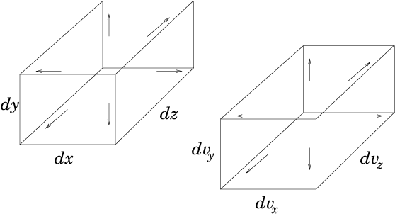
<mrow><mi mathvariant="bold-italic">dx</mi></mrow></math>, see Fig.&nbsp;<a href="chap8.xml#lphasespace">8.1</a>. It is located at the
position <math xmlns="http://www.w3.org/1998/Math/MathML">
<mrow><mi mathvariant="bold-italic">x</mi></mrow></math>. We want a sufficient description of the average
properties of the particles in this element.
<div class="p"><!----></div>
<a id="tth_fIg8.1">
</a>   <img src="figures/phasespaceelement.png" alt="figures/phasespaceelement.png" /><a id="phasespaceelement">
</a>
  
<div style="text-align:center">Figure 8.1: The phase-space element is six-dimensional and selects
    particles that lie in a space element <math xmlns="http://www.w3.org/1998/Math/MathML">
<mrow>
<msup><mrow><mi>d</mi></mrow><mrow><mn>3</mn></mrow>
</msup>
<mi>x</mi></mrow></math> and simultaneously in
    a velocity element <math xmlns="http://www.w3.org/1998/Math/MathML">
<mrow>
<msup><mrow><mi>d</mi></mrow><mrow><mn>3</mn></mrow>
</msup>
<mi>v</mi></mrow></math>.<a id="lphasespace">
</a></div>

<div class="p"><!----></div>
We use a statistical description originally invented by James Clerk
Maxwell called the "distribution function". The distribution
function is a quantity <math xmlns="http://www.w3.org/1998/Math/MathML">
<mrow><mi>f</mi><mo stretchy="false">(</mo><mi mathvariant="bold-italic">v</mi><mo>,</mo><mi mathvariant="bold-italic">x</mi><mo>,</mo><mi>t</mi><mo stretchy="false">)</mo></mrow></math> that is a function of
velocity <math xmlns="http://www.w3.org/1998/Math/MathML">
<mrow><mi mathvariant="bold-italic">v</mi></mrow></math>, position <math xmlns="http://www.w3.org/1998/Math/MathML">
<mrow><mi mathvariant="bold-italic">x</mi></mrow></math>, and time <math xmlns="http://www.w3.org/1998/Math/MathML">
<mrow><mi>t</mi></mrow></math>. The distribution
function is defined by considering an element in
<em>velocity-space</em><a 
id="velocity-space81477"></a> <math xmlns="http://www.w3.org/1998/Math/MathML">
<mrow>
<msup><mrow><mi>d</mi></mrow><mrow><mn>3</mn></mrow>
</msup>
<mi>v</mi><mo>=</mo>
<msub><mrow><mi mathvariant="italic">dv</mi></mrow><mrow><mi>x</mi></mrow>
</msub>
<mo>.</mo>
<msub><mrow><mi mathvariant="italic">dv</mi></mrow><mrow><mi>y</mi></mrow>
</msub>
<mo>.</mo>
<msub><mrow><mi mathvariant="italic">dv</mi></mrow><mrow><mi>z</mi></mrow>
</msub>
</mrow></math> with
sides <math xmlns="http://www.w3.org/1998/Math/MathML">
<mrow><mi mathvariant="bold-italic">dv</mi></mrow></math> located at velocity <math xmlns="http://www.w3.org/1998/Math/MathML">
<mrow><mi mathvariant="bold-italic">v</mi></mrow></math>. Any particle whose
velocity components lie simultaneously in the ranges <math xmlns="http://www.w3.org/1998/Math/MathML">
<mrow>
<msub><mrow><mi>v</mi></mrow><mrow><mi>x</mi></mrow>
</msub>
<mo>&rarr;</mo>
<msub><mrow><mi>v</mi></mrow><mrow><mi>x</mi></mrow>
</msub>
<mo>+</mo>
<msub><mrow><mi mathvariant="italic">dv</mi></mrow><mrow><mi>x</mi></mrow>
</msub>
</mrow></math>, <math xmlns="http://www.w3.org/1998/Math/MathML">
<mrow>
<msub><mrow><mi>v</mi></mrow><mrow><mi>y</mi></mrow>
</msub>
<mo>&rarr;</mo>
<msub><mrow><mi>v</mi></mrow><mrow><mi>y</mi></mrow>
</msub>
<mo>+</mo>
<msub><mrow><mi mathvariant="italic">dv</mi></mrow><mrow><mi>y</mi></mrow>
</msub>
</mrow></math>, <math xmlns="http://www.w3.org/1998/Math/MathML">
<mrow>
<msub><mrow><mi>v</mi></mrow><mrow><mi>z</mi></mrow>
</msub>
<mo>&rarr;</mo>
<msub><mrow><mi>v</mi></mrow><mrow><mi>z</mi></mrow>
</msub>
<mo>+</mo>
<msub><mrow><mi mathvariant="italic">dv</mi></mrow><mrow><mi>z</mi></mrow>
</msub>
</mrow></math>, is inside that
velocity element.

<div class="p"><!----></div>
Then at any time <math xmlns="http://www.w3.org/1998/Math/MathML">
<mrow><mi>t</mi></mrow></math> the distribution function
<math xmlns="http://www.w3.org/1998/Math/MathML">
<mrow><mi>f</mi><mo stretchy="false">(</mo><mi mathvariant="bold-italic">v</mi><mo>,</mo><mi mathvariant="bold-italic">x</mi><mo>,</mo><mi>t</mi><mo stretchy="false">)</mo></mrow></math>, is such that the number of particles in the
spatial element <math xmlns="http://www.w3.org/1998/Math/MathML">
<mrow>
<msup><mrow><mi>d</mi></mrow><mrow><mn>3</mn></mrow>
</msup>
<mi>x</mi></mrow></math> that have velocities in the velocity element
<math xmlns="http://www.w3.org/1998/Math/MathML">
<mrow>
<msup><mrow><mi>d</mi></mrow><mrow><mn>3</mn></mrow>
</msup>
<mi>v</mi></mrow></math> is
<a id="distribfunc">
</a><br />
<table width="100%"><tr><td align="center">
    <math xmlns="http://www.w3.org/1998/Math/MathML">
    <mstyle displaystyle="true"><mrow><mi>f</mi><mo stretchy="false">(</mo><mi mathvariant="bold-italic">v</mi><mo>,</mo><mi mathvariant="bold-italic">x</mi><mo>,</mo><mi>t</mi><mo stretchy="false">)</mo>
<msup><mrow><mi>d</mi></mrow><mrow><mn>3</mn></mrow>
</msup>
<mi>v</mi>
<msup><mrow><mi>d</mi></mrow><mrow><mn>3</mn></mrow>
</msup>
<mi>x</mi><mo>.</mo></mrow>
    </mstyle></math></td><td width="1">
    <math xmlns="http://www.w3.org/1998/Math/MathML">
    <mstyle displaystyle="true"><mrow><mo stretchy="false">(</mo><mn>8</mn><mo>.</mo><mn>1</mn><mo stretchy="false">)</mo></mrow>
    </mstyle></math>
</td></tr></table>


The distribution function is therefore the density of particles in the
six-dimensional "phase-space"<a 
id="phase-space81478"></a> combining velocity
and space. Its utility arises from the presumption that because of the
enormous number of particles in the problem we can let the velocity
and spatial elements, that is the phase-space element <math xmlns="http://www.w3.org/1998/Math/MathML">
<mrow>
<msup><mrow><mi>d</mi></mrow><mrow><mn>3</mn></mrow>
</msup>

<msup><mrow><mi mathvariant="italic">vd</mi></mrow><mrow><mn>3</mn></mrow>
</msup>
<mi>x</mi></mrow></math>,
become almost infinitesimally small and yet still have a large number
of particles in it. With a large number of particles, statistical
descriptions make sense. In particular, it makes sense to think of <math xmlns="http://www.w3.org/1998/Math/MathML">
<mrow><mi>f</mi></mrow></math>
as a kind of continuous fluid in six dimensions. Obviously if the
phase-space element is shrunk down to a sufficiently small size, then
eventually there will be very few particles in it. The
discreteness<a 
id="discreteness_of_particles81479"></a> of the particles becomes
visible and eventually there are either one or no particles in each
tiny volume. But if we can shrink the element enough that it is small
compared with the smallest scales in the problem while it still
contains a large number of particles, then we have a sufficient
statistical description if we know <math xmlns="http://www.w3.org/1998/Math/MathML">
<mrow><mi>f</mi></mrow></math> everywhere, but we don't know
the coordinates of each individual particle.  The most famous of all
such distribution functions is the Maxwellian<a 
id="Maxwell-Boltzmann___distribution81480"></a>, which is
<a id="Maxwellian">
</a><br />
<table width="100%"><tr><td align="center">
    <math xmlns="http://www.w3.org/1998/Math/MathML">
    <mstyle displaystyle="true"><mrow><mi>f</mi><mo stretchy="false">(</mo><mi mathvariant="bold-italic">v</mi><mo>,</mo><mi mathvariant="bold-italic">x</mi><mo>,</mo><mi>t</mi><mo stretchy="false">)</mo><mo>=</mo><mi>n</mi><mo stretchy="false">(</mo><mi mathvariant="bold-italic">x</mi><mo>,</mo><mi>t</mi><mo stretchy="false">)</mo>
<msup><mrow><mo>(</mo>
<mfrac><mrow><mi>m</mi></mrow>
<mrow><mn>2</mn><mi mathvariant="italic">&pi;</mi><mi>k</mi><mi>T</mi></mrow>
</mfrac>
<mo>)</mo></mrow><mrow><mn>3</mn><mo stretchy="false">/</mo><mn>2</mn></mrow>
</msup>
<mi>exp</mi><mrow><mo>(</mo><mo>-</mo>
<mfrac><mrow>
<msup><mrow><mi mathvariant="italic">mv</mi></mrow><mrow><mn>2</mn></mrow>
</msup>
</mrow>
<mrow><mn>2</mn><mi mathvariant="italic">kT</mi></mrow>
</mfrac>
<mo>)</mo></mrow><mo>.</mo></mrow>
    </mstyle></math></td><td width="1">
    <math xmlns="http://www.w3.org/1998/Math/MathML">
    <mstyle displaystyle="true"><mrow><mo stretchy="false">(</mo><mn>8</mn><mo>.</mo><mn>2</mn><mo stretchy="false">)</mo></mrow>
    </mstyle></math>
</td></tr></table>


Here <math xmlns="http://www.w3.org/1998/Math/MathML">
<mrow><mi>m</mi></mrow></math> is the mass of the particles, <math xmlns="http://www.w3.org/1998/Math/MathML">
<mrow><mi>T</mi></mrow></math> their temperature, and <math xmlns="http://www.w3.org/1998/Math/MathML">
<mrow><mi>k</mi></mrow></math>
Boltzmann's constant. The squared velocity
<math xmlns="http://www.w3.org/1998/Math/MathML">
<mrow>
<msup><mrow><mi>v</mi></mrow><mrow><mn>2</mn></mrow>
</msup>
<mo>=</mo><mi mathvariant="bold-italic">v</mi><mo>.</mo><mi mathvariant="bold-italic">v</mi><mo>=</mo>
<msubsup><mrow><mi>v</mi></mrow><mrow><mi>x</mi> </mrow>
<mrow><mn>2</mn></mrow></msubsup>
<mo>+</mo>
<msubsup><mrow><mi>v</mi></mrow><mrow><mi>y</mi> </mrow>
<mrow><mn>2</mn></mrow></msubsup>
<mo>+</mo>
<msubsup><mrow><mi>v</mi></mrow><mrow><mi>z</mi> </mrow>
<mrow><mn>2</mn></mrow></msubsup>
</mrow></math> appearing in the exponential
makes the distributions in the different coordinate directions
separable<a 
id="separable_coordinates81481"></a>
<a id="separategaus">
</a><br />
<table width="100%"><tr><td align="center">
    <math xmlns="http://www.w3.org/1998/Math/MathML">
    <mstyle displaystyle="true"><mrow><mi>exp</mi><mrow><mo>(</mo><mo>-</mo>
<mfrac><mrow>
<msup><mrow><mi mathvariant="italic">mv</mi></mrow><mrow><mn>2</mn></mrow>
</msup>
</mrow>
<mrow><mn>2</mn><mi mathvariant="italic">kT</mi></mrow>
</mfrac>
<mo>)</mo></mrow><mo>=</mo><mi>exp</mi><mrow><mo>(</mo><mo>-</mo>
<mfrac><mrow>
<msubsup><mrow><mi mathvariant="italic">mv</mi></mrow><mrow><mi>x</mi> </mrow>
<mrow><mn>2</mn></mrow></msubsup>
</mrow>
<mrow><mn>2</mn><mi mathvariant="italic">kT</mi></mrow>
</mfrac>
<mo>)</mo></mrow><mi>exp</mi><mrow><mo>(</mo><mo>-</mo>
<mfrac><mrow>
<msubsup><mrow><mi mathvariant="italic">mv</mi></mrow><mrow><mi>y</mi> </mrow>
<mrow><mn>2</mn></mrow></msubsup>
</mrow>
<mrow><mn>2</mn><mi mathvariant="italic">kT</mi></mrow>
</mfrac>
<mo>)</mo></mrow><mi>exp</mi><mrow><mo>(</mo><mo>-</mo>
<mfrac><mrow>
<msubsup><mrow><mi mathvariant="italic">mv</mi></mrow><mrow><mi>z</mi> </mrow>
<mrow><mn>2</mn></mrow></msubsup>
</mrow>
<mrow><mn>2</mn><mi mathvariant="italic">kT</mi></mrow>
</mfrac>
<mo>)</mo></mrow><mo>.</mo></mrow>
    </mstyle></math></td><td width="1">
    <math xmlns="http://www.w3.org/1998/Math/MathML">
    <mstyle displaystyle="true"><mrow><mo stretchy="false">(</mo><mn>8</mn><mo>.</mo><mn>3</mn><mo stretchy="false">)</mo></mrow>
    </mstyle></math>
</td></tr></table>


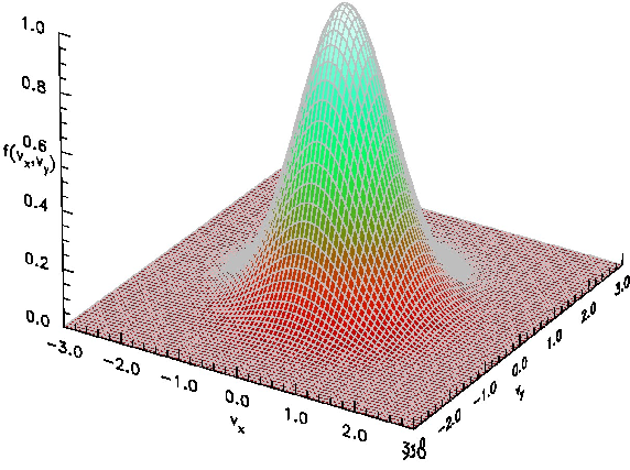
See Fig.&nbsp;<a href="chap8.xml#lmaxwellian">8.2</a>.

<div class="p"><!----></div>
<a id="tth_fIg8.2">
</a>   <img src="figures/maxwellian.png" alt="figures/maxwellian.png" /><a id="maxwellian">
</a>
  
<div style="text-align:center">Figure 8.2: A Maxwellian distribution function in two dimensions
    displayed as a perspective view of the surface <math xmlns="http://www.w3.org/1998/Math/MathML">
<mrow><mi>f</mi><mo stretchy="false">(</mo>
<msub><mrow><mi>v</mi></mrow><mrow><mi>x</mi></mrow>
</msub>
<mo>,</mo>
<msub><mrow><mi>v</mi></mrow><mrow><mi>y</mi></mrow>
</msub>
<mo stretchy="false">)</mo></mrow></math>, with
    velocities <math xmlns="http://www.w3.org/1998/Math/MathML">
<mrow><mo stretchy="false">(</mo>
<msub><mrow><mi>v</mi></mrow><mrow><mi>x</mi></mrow>
</msub>
<mo>,</mo>
<msub><mrow><mi>v</mi></mrow><mrow><mi>y</mi></mrow>
</msub>
<mo stretchy="false">)</mo></mrow></math> normalized to the thermal velocity
    <math xmlns="http://www.w3.org/1998/Math/MathML">
<mrow><msqrt><mrow><mn>2</mn><mi>T</mi><mo stretchy="false">/</mo><mi>m</mi></mrow></msqrt></mrow></math>. This can be considered to be the proportional to
    the distribution at a fixed value of <math xmlns="http://www.w3.org/1998/Math/MathML">
<mrow>
<msub><mrow><mi>v</mi></mrow><mrow><mi>z</mi></mrow>
</msub>
</mrow></math>, since the Maxwellian
    is separable.<a id="lmaxwellian">
</a></div>

<div class="p"><!----></div>
The factor <math xmlns="http://www.w3.org/1998/Math/MathML">
<mrow>
<msup><mrow><mo>(</mo>
<mfrac><mrow><mi>m</mi></mrow>
<mrow><mn>2</mn><mi mathvariant="italic">&pi;</mi><mi mathvariant="italic">kT</mi></mrow>
</mfrac>
<mo>)</mo></mrow><mrow><mn>3</mn><mo stretchy="false">/</mo><mn>2</mn></mrow>
</msup>
</mrow></math> normalizes the
distributions in the three velocity dimensions. It is equal to the
inverse of the integral of eq.&nbsp;(<a href="chap8.xml#separategaus">8.3</a>) over all
velocities. Therefore the leading term <math xmlns="http://www.w3.org/1998/Math/MathML">
<mrow><mi>n</mi><mo stretchy="false">(</mo><mi mathvariant="bold-italic">x</mi><mo>,</mo><mi>t</mi><mo stretchy="false">)</mo></mrow></math> is just the
density in space<a 
id="density81482"></a> (not phase-space). It might vary with
position or time. The Maxwellian distribution is what occurs in
<em>thermodynamic equilibrium</em><a 
id="thermodynamic_equilibrium81483"></a> when
there are no substantial effects driving the velocity distribution
away from its natural form. But there are many important situations
where non-thermal, that is non-Maxwellian, distributions arise.

<div class="p"><!----></div>
The distribution function directly determines the mean flow
velocity<a 
id="flow_velocity81484"></a>, and for particles whose internal energy
is unimportant, the energy 
density<a 
id="density_energy81485"></a><a 
id="energy_density81486"></a>. 
The particle flux density, which is the fluid velocity
times the fluid density, is
<a id="meanvel">
</a><br />
<table width="100%"><tr><td align="center">
    <math xmlns="http://www.w3.org/1998/Math/MathML">
    <mstyle displaystyle="true"><mrow><mi mathvariant="bold-italic">&Gamma;</mi><mo>=</mo><mi>n</mi><mi mathvariant="bold-italic">v</mi><mo>=</mo><mo>&int;</mo><mi mathvariant="bold-italic">v</mi><mi>f</mi><mo stretchy="false">(</mo><mi mathvariant="bold-italic">v</mi><mo>,</mo><mi mathvariant="bold-italic">x</mi><mo>,</mo><mi>t</mi><mo stretchy="false">)</mo>
<msup><mrow><mi>d</mi></mrow><mrow><mn>3</mn></mrow>
</msup>
<mi>v</mi><mo>.</mo></mrow>
    </mstyle></math></td><td width="1">
    <math xmlns="http://www.w3.org/1998/Math/MathML">
    <mstyle displaystyle="true"><mrow><mo stretchy="false">(</mo><mn>8</mn><mo>.</mo><mn>4</mn><mo stretchy="false">)</mo></mrow>
    </mstyle></math>
</td></tr></table>


The kinetic energy density<a 
id="kinetic_energy81487"></a>, which for a
stationary fluid can be considered the density times <math xmlns="http://www.w3.org/1998/Math/MathML">
<mrow><mn>3</mn><mo stretchy="false">/</mo><mn>2</mn></mrow></math> times the
temperature is
<a id="energyden">
</a><br />
<table width="100%"><tr><td align="center">
    <math xmlns="http://www.w3.org/1998/Math/MathML">
    <mstyle displaystyle="true"><mrow><mrow><mstyle fontfamily="helvetica"><mi fontstyle="italic">E</mi></mstyle></mrow>
<mo>=</mo>
<mfrac><mrow><mn>3</mn></mrow>
<mrow><mn>2</mn></mrow>
</mfrac>
<mi>n</mi><mi>k</mi><mi>T</mi><mo>=</mo><mo>&int;</mo>
<mfrac><mrow><mn>1</mn></mrow>
<mrow><mn>2</mn></mrow>
</mfrac>
<mi>m</mi>
<msup><mrow><mi>v</mi></mrow><mrow><mn>2</mn></mrow>
</msup>
<mi>f</mi>
<msup><mrow><mi>d</mi></mrow><mrow><mn>3</mn></mrow>
</msup>
<mi>v</mi><mo>.</mo></mrow>
    </mstyle></math></td><td width="1">
    <math xmlns="http://www.w3.org/1998/Math/MathML">
    <mstyle displaystyle="true"><mrow><mo stretchy="false">(</mo><mn>8</mn><mo>.</mo><mn>5</mn><mo stretchy="false">)</mo></mrow>
    </mstyle></math>
</td></tr></table>


<div class="p"><!----></div>
When the distribution in a specific coordinate direction does not
concern us, perhaps because it is known, or because by symmetry it is
unimportant, we often reduce the number of dimensions which we
track. For example, often we might address only the <math xmlns="http://www.w3.org/1998/Math/MathML">
<mrow><mi>x</mi></mrow></math>-direction
velocity, <math xmlns="http://www.w3.org/1998/Math/MathML">
<mrow>
<msub><mrow><mi>v</mi></mrow><mrow><mi>x</mi></mrow>
</msub>
</mrow></math>. In that case, we use a one-dimensional distribution
function,
<a id="oneddist">
</a><br />
<table width="100%"><tr><td align="center">
    <math xmlns="http://www.w3.org/1998/Math/MathML">
    <mstyle displaystyle="true"><mrow>
<msub><mrow><mi>f</mi></mrow><mrow><mi>x</mi></mrow>
</msub>
<mo stretchy="false">(</mo>
<msub><mrow><mi>v</mi></mrow><mrow><mi>x</mi></mrow>
</msub>
<mo stretchy="false">)</mo><mo>=</mo><mo>&int;</mo><mi>f</mi><mo stretchy="false">(</mo><mi mathvariant="bold-italic">v</mi><mo stretchy="false">)</mo>
<msub><mrow><mi mathvariant="italic">dv</mi></mrow><mrow><mi>y</mi></mrow>
</msub>

<msub><mrow><mi mathvariant="italic">dv</mi></mrow><mrow><mi>z</mi></mrow>
</msub>
<mo>,</mo></mrow>
    </mstyle></math></td><td width="1">
    <math xmlns="http://www.w3.org/1998/Math/MathML">
    <mstyle displaystyle="true"><mrow><mo stretchy="false">(</mo><mn>8</mn><mo>.</mo><mn>6</mn><mo stretchy="false">)</mo></mrow>
    </mstyle></math>
</td></tr></table>


that is the <em>integral</em><a 
id="distribution__1-dimensional81488"></a>
of the full three dimensional distribution
over the ignorable velocity coordinates. In effect, <math xmlns="http://www.w3.org/1998/Math/MathML">
<mrow>
<msub><mrow><mi>f</mi></mrow><mrow><mi>x</mi></mrow>
</msub>
<mo stretchy="false">(</mo>
<msub><mrow><mi>v</mi></mrow><mrow><mi>x</mi></mrow>
</msub>
<mo stretchy="false">)</mo></mrow></math> picks
out a particular <math xmlns="http://www.w3.org/1998/Math/MathML">
<mrow>
<msub><mrow><mi>v</mi></mrow><mrow><mi>x</mi></mrow>
</msub>
</mrow></math> but includes all possible <math xmlns="http://www.w3.org/1998/Math/MathML">
<mrow>
<msub><mrow><mi>v</mi></mrow><mrow><mi>y</mi></mrow>
</msub>
</mrow></math> and <math xmlns="http://www.w3.org/1998/Math/MathML">
<mrow>
<msub><mrow><mi>v</mi></mrow><mrow><mi>z</mi></mrow>
</msub>
</mrow></math>. So
the number of particles in the velocity element <math xmlns="http://www.w3.org/1998/Math/MathML">
<mrow>
<msub><mrow><mi mathvariant="italic">dv</mi></mrow><mrow><mi>x</mi></mrow>
</msub>
</mrow></math> is <math xmlns="http://www.w3.org/1998/Math/MathML">
<mrow>
<msub><mrow><mi>f</mi></mrow><mrow><mi>x</mi></mrow>
</msub>
<mo stretchy="false">(</mo>
<msub><mrow><mi>v</mi></mrow><mrow><mi>x</mi></mrow>
</msub>
<mo stretchy="false">)</mo>
<msub><mrow><mi mathvariant="italic">dv</mi></mrow><mrow><mi>x</mi></mrow>
</msub>
</mrow></math>.

<div class="p"><!----></div>
The distribution function first arose in connection with the kinetic
theory of gases<a 
id="kinetic_theory81489"></a>. Its use is therefore often
referred to as "kinetic theory".

<div class="p"><!----></div>
 <a id="tth_sEc8.2"></a><h2>
8.2&nbsp;&nbsp;Conservation of Particles in Phase-Space</h2>

<div class="p"><!----></div>
<a 
id="Boltzmann_equation82490"></a> Boltzmann's equation governs the
conservation of particles; not just in space, which is the continuity
equation (<a href="chap4.xml#continuity">4.5</a>)<a 
id="particle___conservation82491"></a><a 
id="conservation_particles82492"></a>, but in
phase-space. When solved, it tells us what the distribution function
actually is. Its derivation is mathematically very much like the
derivation of the fluid continuity equation. The main complication is
that one needs to think in six dimensions! We'll usually illustrate
this thinking in a (2-dimensional) diagram, using just one space (<math xmlns="http://www.w3.org/1998/Math/MathML">
<mrow><mi>x</mi></mrow></math>
as the abscissa) and one velocity (<math xmlns="http://www.w3.org/1998/Math/MathML">
<mrow><mi>v</mi></mrow></math> as the ordinate) dimension.
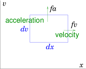
See Fig.&nbsp;<a href="chap8.xml#phasespacefluxl">8.3</a>.

<div class="p"><!----></div>
<a id="tth_fIg8.3">
</a>   <img src="figures/phasespaceflux.png" alt="figures/phasespaceflux.png" /><a id="phasespaceflux">
</a>
  
<div style="text-align:center">Figure 8.3: In phase-space, velocity <math xmlns="http://www.w3.org/1998/Math/MathML">
<mrow><mi>v</mi></mrow></math> carries a particle in the
    <math xmlns="http://www.w3.org/1998/Math/MathML">
<mrow><mi>x</mi></mrow></math>-direction, acceleration carries it in the
    <math xmlns="http://www.w3.org/1998/Math/MathML">
<mrow><mi>v</mi></mrow></math>-direction. Particle flux out of an element <math xmlns="http://www.w3.org/1998/Math/MathML">
<mrow><mi mathvariant="italic">dvdx</mi></mrow></math> arises from
    the divergence of the fluxes <math xmlns="http://www.w3.org/1998/Math/MathML">
<mrow><mi mathvariant="italic">fv</mi></mrow></math> and <math xmlns="http://www.w3.org/1998/Math/MathML">
<mrow><mi mathvariant="italic">fa</mi></mrow></math> in the respective
    directions<a id="phasespacefluxl">
</a></div>

<div class="p"><!----></div>
As time passes, particles move in phase-space. The rate of change of
<math xmlns="http://www.w3.org/1998/Math/MathML">
<mrow><mi>x</mi></mrow></math> is the velocity <math xmlns="http://www.w3.org/1998/Math/MathML">
<mrow><mi mathvariant="italic">dx</mi><mo stretchy="false">/</mo><mi mathvariant="italic">dt</mi><mo>=</mo><mi>v</mi></mrow></math>. The rate of change of velocity <math xmlns="http://www.w3.org/1998/Math/MathML">
<mrow><mi>v</mi></mrow></math> is
acceleration <math xmlns="http://www.w3.org/1998/Math/MathML">
<mrow><mi mathvariant="italic">dv</mi><mo stretchy="false">/</mo><mi mathvariant="italic">dt</mi><mo>=</mo><mi>a</mi></mrow></math>. Generally acceleration arises from force (per
particle) divided by particle mass. The force might be gravity, or
(for charged particles) electric or magnetic field. An individual
particle thus moves through the phase-space (in the <math xmlns="http://www.w3.org/1998/Math/MathML">
<mrow><mi mathvariant="italic">xv</mi></mrow></math> plane of our
diagram). If we therefore consider some phase-space volume we can
write the conservation of particles within it just as we did for the
fluid continuity equation as
<a id="pfcontinuity">
</a><br />
<table width="100%"><tr><td align="center">
    <math xmlns="http://www.w3.org/1998/Math/MathML">
    <mstyle displaystyle="true"><mrow>
<mfrac><mrow><mo>&part;</mo><mi>f</mi></mrow>
<mrow><mo>&part;</mo><mi>t</mi></mrow>
</mfrac>
<mo>+</mo>
<msub><mrow><mo>&nabla;</mo></mrow><mrow><mi mathvariant="italic">ps</mi></mrow>
</msub>
<mo>.</mo><mo stretchy="false">(</mo><mi>f</mi>
<msub><mrow><mi mathvariant="bold-italic">v</mi></mrow><mrow><mi mathvariant="italic">ps</mi></mrow>
</msub>
<mo stretchy="false">)</mo><mo>=</mo>
<mfrac><mrow><mo>&part;</mo><mi>f</mi></mrow>
<mrow><mo>&part;</mo><mi>t</mi></mrow>
</mfrac>
<mo>+</mo>
<mfrac><mrow><mo>&part;</mo></mrow>
<mrow><mo>&part;</mo><mi mathvariant="bold-italic">x</mi></mrow>
</mfrac>
<mo>.</mo><mo stretchy="false">(</mo><mi>f</mi><mi mathvariant="bold-italic">v</mi><mo stretchy="false">)</mo><mo>+</mo>
<mfrac><mrow><mo>&part;</mo></mrow>
<mrow><mo>&part;</mo><mi mathvariant="bold-italic">v</mi></mrow>
</mfrac>
<mo>.</mo><mo stretchy="false">(</mo><mi>f</mi><mi mathvariant="bold-italic">a</mi><mo stretchy="false">)</mo><mo>=</mo><mi>S</mi><mo>.</mo></mrow>
    </mstyle></math></td><td width="1">
    <math xmlns="http://www.w3.org/1998/Math/MathML">
    <mstyle displaystyle="true"><mrow><mo stretchy="false">(</mo><mn>8</mn><mo>.</mo><mn>7</mn><mo stretchy="false">)</mo></mrow>
    </mstyle></math>
</td></tr></table>


Here <math xmlns="http://www.w3.org/1998/Math/MathML">
<mrow>
<msub><mrow><mi mathvariant="bold-italic">v</mi></mrow><mrow><mi mathvariant="italic">ps</mi></mrow>
</msub>
</mrow></math> is the "phase-space velocity", a six-dimensional
vector consisting of the combination of the velocity in space and the
acceleration. And <math xmlns="http://www.w3.org/1998/Math/MathML">
<mrow>
<msub><mrow><mo>&nabla;</mo></mrow><mrow><mi mathvariant="italic">ps</mi></mrow>
</msub>
</mrow></math> is the gradient operator in phase
space, likewise a six-dimensional vector. 
<a id="6dphasespace">
</a><br />
<table width="100%"><tr><td align="center">
    <math xmlns="http://www.w3.org/1998/Math/MathML">
    <mstyle displaystyle="true"><mrow>
<msub><mrow><mi mathvariant="bold-italic">v</mi></mrow><mrow><mi mathvariant="italic">ps</mi></mrow>
</msub>
<mo>=</mo><mrow><mo>(</mo>
<mfrac linethickness="0"><mrow><mi mathvariant="bold-italic">v</mi></mrow>
<mrow><mi mathvariant="bold-italic">a</mi></mrow>
</mfrac>
<mo>)</mo></mrow><mo>=</mo><mrow><mo>(</mo>
<mtable>
<mtr><mtd columnalign="center"><mrow>
<msub><mrow><mi>v</mi></mrow><mrow><mi>x</mi></mrow>
</msub>
</mrow></mtd></mtr>
<mtr><mtd columnalign="center"><mrow>
<msub><mrow><mi>v</mi></mrow><mrow><mi>y</mi></mrow>
</msub>
</mrow></mtd></mtr>
<mtr><mtd columnalign="center"><mrow>
<msub><mrow><mi>v</mi></mrow><mrow><mi>z</mi></mrow>
</msub>
</mrow></mtd></mtr>
<mtr><mtd columnalign="center"><mrow>
<msub><mrow><mi>a</mi></mrow><mrow><mi>x</mi></mrow>
</msub>
</mrow></mtd></mtr>
<mtr><mtd columnalign="center"><mrow>
<msub><mrow><mi>a</mi></mrow><mrow><mi>y</mi></mrow>
</msub>
</mrow></mtd></mtr>
<mtr><mtd columnalign="center"><mrow>
<msub><mrow><mi>a</mi></mrow><mrow><mi>z</mi></mrow>
</msub>
</mrow></mtd></mtr></mtable>

<mo>)</mo></mrow><mo>,</mo><mi>&ensp;</mi>
<mtext>and</mtext>
<mi>&ensp;</mi>
<msub><mrow><mo mathvariant="bold-italic">&nabla;</mo></mrow><mrow><mi mathvariant="italic">ps</mi></mrow>
</msub>
<mo>=</mo><mrow><mo>(</mo>
<mfrac linethickness="0"><mrow><mo mathvariant="bold-italic">&nabla;</mo></mrow>
<mrow>
<msub><mrow><mo mathvariant="bold-italic">&nabla;</mo></mrow><mrow><mi>v</mi></mrow>
</msub>
</mrow>
</mfrac>
<mo>)</mo></mrow><mo>=</mo><mrow><mo>(</mo>
<mfrac linethickness="0"><mrow>
<mfrac><mrow><mo>&part;</mo></mrow>
<mrow><mo>&part;</mo><mi mathvariant="bold-italic">x</mi></mrow>
</mfrac>
</mrow>
<mrow>
<mfrac><mrow><mo>&part;</mo></mrow>
<mrow><mo>&part;</mo><mi mathvariant="bold-italic">v</mi></mrow>
</mfrac>
</mrow>
</mfrac>
<mo>)</mo></mrow><mo>=</mo><mrow><mo>(</mo>
<mtable>
<mtr><mtd columnalign="center"><mrow><mo>&part;</mo><mo stretchy="false">/</mo><mo>&part;</mo><mi>x</mi></mrow></mtd></mtr>
<mtr><mtd columnalign="center"><mrow><mo>&part;</mo><mo stretchy="false">/</mo><mo>&part;</mo><mi>y</mi></mrow></mtd></mtr>
<mtr><mtd columnalign="center"><mrow><mo>&part;</mo><mo stretchy="false">/</mo><mo>&part;</mo><mi>z</mi></mrow></mtd></mtr>
<mtr><mtd columnalign="center"><mrow><mo>&part;</mo><mo stretchy="false">/</mo><mo>&part;</mo>
<msub><mrow><mi>v</mi></mrow><mrow><mi>x</mi></mrow>
</msub>
</mrow></mtd></mtr>
<mtr><mtd columnalign="center"><mrow><mo>&part;</mo><mo stretchy="false">/</mo><mo>&part;</mo>
<msub><mrow><mi>v</mi></mrow><mrow><mi>y</mi></mrow>
</msub>
</mrow></mtd></mtr>
<mtr><mtd columnalign="center"><mrow><mo>&part;</mo><mo stretchy="false">/</mo><mo>&part;</mo>
<msub><mrow><mi>v</mi></mrow><mrow><mi>z</mi></mrow>
</msub>
</mrow></mtd></mtr></mtable>

<mo>)</mo></mrow><mo>.</mo></mrow>
    </mstyle></math></td><td width="1">
    <math xmlns="http://www.w3.org/1998/Math/MathML">
    <mstyle displaystyle="true"><mrow><mo stretchy="false">(</mo><mn>8</mn><mo>.</mo><mn>8</mn><mo stretchy="false">)</mo></mrow>
    </mstyle></math>
</td></tr></table>


The notation most usually used is to write out the space and velocity
parts of the derivatives separately.
<a id="spatialderivatives">
</a><br />
<table width="100%"><tr><td align="center">
    <math xmlns="http://www.w3.org/1998/Math/MathML">
    <mstyle displaystyle="true"><mrow>
<mfrac><mrow><mo>&part;</mo></mrow>
<mrow><mo>&part;</mo><mi mathvariant="bold-italic">x</mi></mrow>
</mfrac>
<mo>.</mo><mo stretchy="false">(</mo><mi>f</mi><mi mathvariant="bold-italic">v</mi><mo stretchy="false">)</mo><mo>=</mo>
<mfrac><mrow><mo>&part;</mo><mo stretchy="false">(</mo><mi>f</mi>
<msub><mrow><mi>v</mi></mrow><mrow><mi>x</mi></mrow>
</msub>
<mo stretchy="false">)</mo></mrow>
<mrow><mo>&part;</mo><mi>x</mi></mrow>
</mfrac>
<mo>+</mo>
<mfrac><mrow><mo>&part;</mo><mo stretchy="false">(</mo><mi>f</mi>
<msub><mrow><mi>v</mi></mrow><mrow><mi>y</mi></mrow>
</msub>
<mo stretchy="false">)</mo></mrow>
<mrow><mo>&part;</mo><mi>y</mi></mrow>
</mfrac>
<mo>+</mo>
<mfrac><mrow><mo>&part;</mo><mo stretchy="false">(</mo><mi>f</mi>
<msub><mrow><mi>v</mi></mrow><mrow><mi>z</mi></mrow>
</msub>
<mo stretchy="false">)</mo></mrow>
<mrow><mo>&part;</mo><mi>z</mi></mrow>
</mfrac>
</mrow>
    </mstyle></math></td><td width="1">
    <math xmlns="http://www.w3.org/1998/Math/MathML">
    <mstyle displaystyle="true"><mrow><mo stretchy="false">(</mo><mn>8</mn><mo>.</mo><mn>9</mn><mo stretchy="false">)</mo></mrow>
    </mstyle></math>
</td></tr></table>


and
<a id="velocityderivatives">
</a><br />
<table width="100%"><tr><td align="center">
    <math xmlns="http://www.w3.org/1998/Math/MathML">
    <mstyle displaystyle="true"><mrow>
<mfrac><mrow><mo>&part;</mo></mrow>
<mrow><mo>&part;</mo><mi mathvariant="bold-italic">v</mi></mrow>
</mfrac>
<mo>.</mo><mo stretchy="false">(</mo><mi>f</mi><mi mathvariant="bold-italic">a</mi><mo stretchy="false">)</mo><mo>=</mo>
<mfrac><mrow><mo>&part;</mo><mo stretchy="false">(</mo><mi>f</mi>
<msub><mrow><mi>a</mi></mrow><mrow><mi>x</mi></mrow>
</msub>
<mo stretchy="false">)</mo></mrow>
<mrow><mo>&part;</mo>
<msub><mrow><mi>v</mi></mrow><mrow><mi>x</mi></mrow>
</msub>
</mrow>
</mfrac>
<mo>+</mo>
<mfrac><mrow><mo>&part;</mo><mo stretchy="false">(</mo><mi>f</mi>
<msub><mrow><mi>a</mi></mrow><mrow><mi>y</mi></mrow>
</msub>
<mo stretchy="false">)</mo></mrow>
<mrow><mo>&part;</mo>
<msub><mrow><mi>v</mi></mrow><mrow><mi>y</mi></mrow>
</msub>
</mrow>
</mfrac>
<mo>+</mo>
<mfrac><mrow><mo>&part;</mo><mo stretchy="false">(</mo><mi>f</mi>
<msub><mrow><mi>a</mi></mrow><mrow><mi>z</mi></mrow>
</msub>
<mo stretchy="false">)</mo></mrow>
<mrow><mo>&part;</mo>
<msub><mrow><mi>v</mi></mrow><mrow><mi>z</mi></mrow>
</msub>
</mrow>
</mfrac>
<mo>.</mo></mrow>
    </mstyle></math></td><td width="1">
    <math xmlns="http://www.w3.org/1998/Math/MathML">
    <mstyle displaystyle="true"><mrow><mo stretchy="false">(</mo><mn>8</mn><mo>.</mo><mn>10</mn><mo stretchy="false">)</mo></mrow>
    </mstyle></math>
</td></tr></table>


This helps us remember we are dealing with phase-space. Equation
(<a href="chap8.xml#pfcontinuity">8.7</a>) expresses the fact that the rate of change of
number particles in a phase-space element is equal to the rate at
which they are flowing inward across its boundary plus the combined
source rate inside the element, <math xmlns="http://www.w3.org/1998/Math/MathML">
<mrow><mi>S</mi></mrow></math> (all per unit volume). Particles
flow across the boundary either by moving in space across the boundary
of <math xmlns="http://www.w3.org/1998/Math/MathML">
<mrow>
<msup><mrow><mi>d</mi></mrow><mrow><mn>3</mn></mrow>
</msup>
<mi>x</mi></mrow></math>, or by accelerating (moving in velocity-space) across the
boundary of <math xmlns="http://www.w3.org/1998/Math/MathML">
<mrow>
<msup><mrow><mi>d</mi></mrow><mrow><mn>3</mn></mrow>
</msup>
<mi>v</mi></mrow></math>.

<div class="p"><!----></div>
A final simplification arises in eq.&nbsp;(<a href="chap8.xml#pfcontinuity">8.7</a>) because of
what a partial derivative means. It means take the derivative
<em>keeping all the other phase-space coordinates constant</em>. In
other words, the partial <math xmlns="http://www.w3.org/1998/Math/MathML">
<mrow><mi>x</mi></mrow></math>-derivative holds <math xmlns="http://www.w3.org/1998/Math/MathML">
<mrow><mi>y</mi><mo>,</mo><mi>z</mi><mo>,</mo>
<msub><mrow><mi>v</mi></mrow><mrow><mi>x</mi></mrow>
</msub>
<mo>,</mo>
<msub><mrow><mi>v</mi></mrow><mrow><mi>y</mi></mrow>
</msub>
<mo>,</mo>
<msub><mrow><mi>v</mi></mrow><mrow><mi>z</mi></mrow>
</msub>
</mrow></math>
constant. The partial derivative of any <math xmlns="http://www.w3.org/1998/Math/MathML">
<mrow>
<msub><mrow><mi>v</mi></mrow><mrow><mi>j</mi></mrow>
</msub>
</mrow></math> with respect to any
<math xmlns="http://www.w3.org/1998/Math/MathML">
<mrow>
<msub><mrow><mi>x</mi></mrow><mrow><mi>k</mi></mrow>
</msub>
</mrow></math> is therefore zero, which means that in the spatial divergence
eq.&nbsp;(<a href="chap8.xml#spatialderivatives">8.9</a>) the velocity factors can be taken
outside the spatial derivatives to write
<a id="spatialdivergence">
</a><br />
<table width="100%"><tr><td align="center">
    <math xmlns="http://www.w3.org/1998/Math/MathML">
    <mstyle displaystyle="true"><mrow>
<mfrac><mrow><mo>&part;</mo></mrow>
<mrow><mo>&part;</mo><mi mathvariant="bold-italic">x</mi></mrow>
</mfrac>
<mo>.</mo><mo stretchy="false">(</mo><mi>f</mi><mi mathvariant="bold-italic">v</mi><mo stretchy="false">)</mo><mo>=</mo><mi mathvariant="bold-italic">v</mi><mo>.</mo>
<mfrac><mrow><mo>&part;</mo><mi>f</mi></mrow>
<mrow><mo>&part;</mo><mi mathvariant="bold-italic">x</mi></mrow>
</mfrac>
<mo>=</mo>
<msub><mrow><mi>v</mi></mrow><mrow><mi>x</mi></mrow>
</msub>

<mfrac><mrow><mo>&part;</mo><mi>f</mi></mrow>
<mrow><mo>&part;</mo><mi>x</mi></mrow>
</mfrac>
<mo>+</mo>
<msub><mrow><mi>v</mi></mrow><mrow><mi>y</mi></mrow>
</msub>

<mfrac><mrow><mo>&part;</mo><mi>f</mi></mrow>
<mrow><mo>&part;</mo><mi>y</mi></mrow>
</mfrac>
<mo>+</mo>
<msub><mrow><mi>v</mi></mrow><mrow><mi>z</mi></mrow>
</msub>

<mfrac><mrow><mo>&part;</mo><mi>f</mi></mrow>
<mrow><mo>&part;</mo><mi>z</mi></mrow>
</mfrac>
<mo>.</mo></mrow>
    </mstyle></math></td><td width="1">
    <math xmlns="http://www.w3.org/1998/Math/MathML">
    <mstyle displaystyle="true"><mrow><mo stretchy="false">(</mo><mn>8</mn><mo>.</mo><mn>11</mn><mo stretchy="false">)</mo></mrow>
    </mstyle></math>
</td></tr></table>


That rearrangement is always possible. If the acceleration of a
particle does not depend on its velocity (or depends on it in such a
way that <math xmlns="http://www.w3.org/1998/Math/MathML">
<mrow>
<msub><mrow><mo>&nabla;</mo></mrow><mrow><mi>v</mi></mrow>
</msub>
<mo>.</mo><mi mathvariant="bold-italic">a</mi><mo>=</mo><mn>0</mn></mrow></math>, which is the case for the Lorentz
force) then we can do the same for the acceleration term.

<div class="p"><!----></div>
Then we arrive at Boltzmann's equation<a 
id="Boltzmann_equation82493"></a>
<a id="Boltzmann">
</a><br />
<table width="100%"><tr><td align="center">
    <math xmlns="http://www.w3.org/1998/Math/MathML">
    <mstyle displaystyle="true"><mrow>
<mfrac><mrow><mo>&part;</mo><mi>f</mi></mrow>
<mrow><mo>&part;</mo><mi>t</mi></mrow>
</mfrac>
<mo>+</mo><mi mathvariant="bold-italic">v</mi><mo>.</mo>
<mfrac><mrow><mo>&part;</mo><mi>f</mi></mrow>
<mrow><mo>&part;</mo><mi mathvariant="bold-italic">x</mi></mrow>
</mfrac>
<mo>+</mo><mi mathvariant="bold-italic">a</mi><mo>.</mo>
<mfrac><mrow><mo>&part;</mo><mi>f</mi></mrow>
<mrow><mo>&part;</mo><mi mathvariant="bold-italic">v</mi></mrow>
</mfrac>
<mo>=</mo><mi>S</mi><mo>=</mo><mi>C</mi><mo>.</mo></mrow>
    </mstyle></math></td><td width="1">
    <math xmlns="http://www.w3.org/1998/Math/MathML">
    <mstyle displaystyle="true"><mrow><mo stretchy="false">(</mo><mn>8</mn><mo>.</mo><mn>12</mn><mo stretchy="false">)</mo></mrow>
    </mstyle></math>
</td></tr></table>


The source term on the right hand side of Boltzmann's equation
contains not only literal creation<a 
id="particle_creation82494"></a> or
destruction of particles (e.g.&nbsp;by chemical or nuclear reactions), but
also any instantaneous changes of velocity, in other words
<em>collisions</em>. A collision<a 
id="collision82495"></a> that does not destroy
or create a particle of the type we are tracking can nevertheless
change its velocity abruptly<a href="footnote.xml#tthFtNtAEF" id="tthFrefAEF"><math xmlns="http://www.w3.org/1998/Math/MathML">
<mrow>
<msup><mrow></mrow><mrow><mn>45</mn></mrow>
</msup>
</mrow></math></a>. This change in
velocity immediately transports the particle from one velocity to
another. The particle jumps to a different position in
phase-space. That constitutes a "sink" at the old velocity and a
"source" at the new velocity. Chemical or nuclear reactions also
occur as a result of collisions, of course. Consequently essentially
all the phenomena that contribute to the Boltzmann equation's source
(with the exception of spontaneous - e.g.&nbsp;radioactive - decay of
the particles) are collisions; and the source term is usually called
the "collision" term and written <math xmlns="http://www.w3.org/1998/Math/MathML">
<mrow><mi>C</mi></mrow></math> instead of <math xmlns="http://www.w3.org/1998/Math/MathML">
<mrow><mi>S</mi></mrow></math>.

<div class="p"><!----></div>
The collision term <math xmlns="http://www.w3.org/1998/Math/MathML">
<mrow><mi>C</mi><mo stretchy="false">(</mo><mi mathvariant="bold-italic">v</mi><mo>,</mo><mi mathvariant="bold-italic">x</mi><mo>,</mo><mi>t</mi><mo stretchy="false">)</mo></mrow></math> is the rate per unit
phase-space-volume of generation (or removal if it is negative) of
particles at position <math xmlns="http://www.w3.org/1998/Math/MathML">
<mrow><mi mathvariant="bold-italic">x</mi></mrow></math> having velocity <math xmlns="http://www.w3.org/1998/Math/MathML">
<mrow><mi mathvariant="bold-italic">v</mi></mrow></math>. It
naturally depends also upon the distribution function <math xmlns="http://www.w3.org/1998/Math/MathML">
<mrow><mi>f</mi></mrow></math> itself. For
example the rate per unit volume at which collisions occur removing
particles of a certain velocity is proportional to the number of such
particles present in the first place.

<div class="p"><!----></div>
 <a id="tth_sEc8.3"></a><h2>
8.3&nbsp;&nbsp;Solving the Hyperbolic Boltzmann Equation</h2>

<div class="p"><!----></div>
     <a id="tth_sEc8.3.1"></a><h3>
8.3.1&nbsp;&nbsp;Integration along orbits</h3>

<div class="p"><!----></div>
<a 
id="orbit83496"></a><a 
id="integration_along_orbit83497"></a>If we know the collision term <math xmlns="http://www.w3.org/1998/Math/MathML">
<mrow><mi>C</mi></mrow></math>, as well as <math xmlns="http://www.w3.org/1998/Math/MathML">
<mrow><mi mathvariant="bold-italic">a</mi></mrow></math>, then clearly
Boltzmann's equation is a first-order linear partial differential
equation (in seven total dimensions including time, or less if there
are ignorable coordinates).  Since it is first order linear with a
single scalar dependent variable<a href="footnote.xml#tthFtNtAEG" id="tthFrefAEG"><math xmlns="http://www.w3.org/1998/Math/MathML">
<mrow>
<msup><mrow></mrow><mrow><mn>46</mn></mrow>
</msup>
</mrow></math></a>, <math xmlns="http://www.w3.org/1998/Math/MathML">
<mrow><mi>f</mi></mrow></math>, it is hyperbolic. That means
we may solve it as an initial value problem<a 
id="hyperbolic83498"></a>.

<div class="p"><!----></div>
The most natural way to do this is to follow particle
trajectories<a 
id="trajectory83499"></a> in phase-space, which we will call
particle orbits. Any individual particle moves in accordance with
<a id="orbitaccel">
</a><br />
<table width="100%"><tr><td align="center">
    <math xmlns="http://www.w3.org/1998/Math/MathML">
    <mstyle displaystyle="true"><mrow>
<mfrac><mrow><mi>d</mi><mi mathvariant="bold-italic">x</mi></mrow>
<mrow><mi>d</mi><mi>t</mi></mrow>
</mfrac>
<mo>=</mo><mi mathvariant="bold-italic">v</mi><mo>,</mo><mi>&emsp;&emsp;&emsp;&emsp;&emsp;&emsp;</mi>
<mfrac><mrow><mi>d</mi><mi mathvariant="bold-italic">v</mi></mrow>
<mrow><mi>d</mi><mi>t</mi></mrow>
</mfrac>
<mo>=</mo><mi mathvariant="bold-italic">a</mi><mo>;</mo><mi>&emsp;&emsp;&emsp;&emsp;&emsp;&emsp;</mi>
<mtext>i.e.</mtext>
<mi>&emsp;&emsp;&emsp;</mi>
<mfrac><mrow><mi>d</mi></mrow>
<mrow><mi>d</mi><mi>t</mi></mrow>
</mfrac>
<mrow><mo>(</mo>
<mfrac linethickness="0"><mrow><mi mathvariant="bold-italic">x</mi></mrow>
<mrow><mi mathvariant="bold-italic">v</mi></mrow>
</mfrac>
<mo>)</mo></mrow><mo>=</mo><mrow><mo>(</mo>
<mfrac linethickness="0"><mrow><mi mathvariant="bold-italic">v</mi></mrow>
<mrow><mi mathvariant="bold-italic">a</mi></mrow>
</mfrac>
<mo>)</mo></mrow></mrow>
    </mstyle></math></td><td width="1">
    <math xmlns="http://www.w3.org/1998/Math/MathML">
    <mstyle displaystyle="true"><mrow><mo stretchy="false">(</mo><mn>8</mn><mo>.</mo><mn>13</mn><mo stretchy="false">)</mo></mrow>
    </mstyle></math>
</td></tr></table>


This is an ordinary differential equation, which we know how to solve
(assuming <math xmlns="http://www.w3.org/1998/Math/MathML">
<mrow><mi mathvariant="bold-italic">a</mi></mrow></math> is known), starting from some initial position in
phase-space <math xmlns="http://www.w3.org/1998/Math/MathML">
<mrow>
<msub><mrow><mi mathvariant="bold-italic">x</mi></mrow><mrow><mn>0</mn></mrow>
</msub>
</mrow></math>, <math xmlns="http://www.w3.org/1998/Math/MathML">
<mrow>
<msub><mrow><mi mathvariant="bold-italic">v</mi></mrow><mrow><mn>0</mn></mrow>
</msub>
</mrow></math>. But how does this orbit help us to
solve Boltzmann's equation for the distribution function? It helps us
because Boltzmann's equation is an equation for the rate of change of
<math xmlns="http://www.w3.org/1998/Math/MathML">
<mrow><mi>f</mi></mrow></math> moving along a particle phase-space orbit.

<div class="p"><!----></div>
Suppose we catch a six-dimensional ride on one of the particles and
move with it, looking out into the phase-space near to us and
measuring the particle density there; watching it change as time goes
by. The rate of change of the distribution function will be precisely
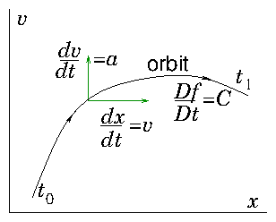
that given by the left hand side of Boltzmann's equation. See Fig.&nbsp;<a href="chap8.xml#phaseorbitl">8.4</a> for a visualization.

<div class="p"><!----></div>
<a id="tth_fIg8.4">
</a>   <img src="figures/phaseorbit.png" alt="figures/phaseorbit.png" /><a id="phaseorbit">
</a>
  
<div style="text-align:center">Figure 8.4: A phase-space orbit is determined by a first order ordinary
    differential equation. The Boltzmann equation states that the rate
    of change of the distribution function along phase-space orbits is
    equal to the collision term.<a id="phaseorbitl">
</a></div>

<div class="p"><!----></div>
First let's convince ourselves that is true. If, during our ride, we
measure the difference in <math xmlns="http://www.w3.org/1998/Math/MathML">
<mrow><mi>f</mi></mrow></math> between times different by a small
interval <math xmlns="http://www.w3.org/1998/Math/MathML">
<mrow><mi mathvariant="italic">dt</mi></mrow></math>. The <math xmlns="http://www.w3.org/1998/Math/MathML">
<mrow><mi>f</mi></mrow></math> will be different because (1) it may have
intrinsic variation with time, resulting in a change <math xmlns="http://www.w3.org/1998/Math/MathML">
<mrow><mi mathvariant="italic">dt</mi><mi>&ensp;</mi><mo>&part;</mo><mi>f</mi><mo stretchy="false">/</mo><mo>&part;</mo><mi>t</mi></mrow></math>; (2) it may have variation with space so our motion has
carried us a distance <math xmlns="http://www.w3.org/1998/Math/MathML">
<mrow><mi mathvariant="italic">dt</mi><mi>&ensp;</mi><mi mathvariant="bold-italic">v</mi></mrow></math>, to a place where <math xmlns="http://www.w3.org/1998/Math/MathML">
<mrow><mi>f</mi></mrow></math> is different
by <math xmlns="http://www.w3.org/1998/Math/MathML">
<mrow><mi mathvariant="italic">dt</mi><mi>&ensp;</mi><mi mathvariant="bold-italic">v</mi><mo>.</mo><mo>&part;</mo><mi>f</mi><mo stretchy="false">/</mo><mo>&part;</mo><mi mathvariant="bold-italic">x</mi></mrow></math>; or (3) it may have
variation with velocity so our motion in velocity space (acceleration)
has carried us a velocity-"distance", <math xmlns="http://www.w3.org/1998/Math/MathML">
<mrow><mi mathvariant="italic">dt</mi><mi>&ensp;</mi><mi mathvariant="bold-italic">a</mi></mrow></math>, to where <math xmlns="http://www.w3.org/1998/Math/MathML">
<mrow><mi>f</mi></mrow></math> is
different by <math xmlns="http://www.w3.org/1998/Math/MathML">
<mrow><mi mathvariant="italic">dt</mi><mi>&ensp;</mi><mi mathvariant="bold-italic">a</mi><mo>.</mo><mo>&part;</mo><mi>f</mi><mo stretchy="false">/</mo><mo>&part;</mo><mi mathvariant="bold-italic">v</mi></mrow></math>.  The total of
these three, divided by <math xmlns="http://www.w3.org/1998/Math/MathML">
<mrow><mi mathvariant="italic">dt</mi></mrow></math>, is the rate of change of <math xmlns="http://www.w3.org/1998/Math/MathML">
<mrow><mi>f</mi></mrow></math> along the
orbit. That's the left hand side of eq.&nbsp;(<a href="chap8.xml#Boltzmann">8.12</a>).

<div class="p"><!----></div>
Second, why is this identity with the total derivative the case? It is
because the flow in phase-space is<a 
id="phase-space_divergence83500"></a>
<em>divergenceless</em><a 
id="divergenceless83501"></a>,
<math xmlns="http://www.w3.org/1998/Math/MathML">
<mrow>
<msub><mrow><mo>&nabla;</mo></mrow><mrow><mi mathvariant="italic">ps</mi></mrow>
</msub>
<mo>.</mo>
<msub><mrow><mi mathvariant="bold-italic">v</mi></mrow><mrow><mi mathvariant="italic">ps</mi></mrow>
</msub>
<mo>=</mo><mn>0</mn></mrow></math>. Just as for an ordinary
three-dimensional fluid for which <math xmlns="http://www.w3.org/1998/Math/MathML">
<mrow><mo>&nabla;</mo><mo>.</mo><mo stretchy="false">(</mo><mi mathvariant="italic">&rho;</mi><mi mathvariant="bold-italic">v</mi><mo stretchy="false">)</mo><mo>=</mo><mi mathvariant="bold-italic">v</mi><mo>.</mo><mo>&nabla;</mo><mi mathvariant="italic">&rho;</mi></mrow></math> if <math xmlns="http://www.w3.org/1998/Math/MathML">
<mrow><mo>&nabla;</mo><mo>.</mo><mi mathvariant="bold-italic">v</mi><mo>=</mo><mn>0</mn></mrow></math>, implying <math xmlns="http://www.w3.org/1998/Math/MathML">
<mrow><mi>D</mi><mi mathvariant="italic">&rho;</mi><mo stretchy="false">/</mo><mi mathvariant="italic">Dt</mi><mo>=</mo><mi>S</mi></mrow></math>,
similarly for a dimensionless flow in phase-space. The phase-space
flow is divergenceless if the acceleration has the requisite property
<math xmlns="http://www.w3.org/1998/Math/MathML">
<mrow>
<msub><mrow><mo>&nabla;</mo></mrow><mrow><mi>v</mi></mrow>
</msub>
<mo>.</mo><mi mathvariant="bold-italic">a</mi><mo>=</mo><mn>0</mn></mrow></math>. This can be interpreted as a statement that
there is no dissipation.

<div class="p"><!----></div>
Third, how does this identity help us? It reduces Boltzmann's
equation to an ordinary differential equation along the
orbits. Writing the total differential as <math xmlns="http://www.w3.org/1998/Math/MathML">
<mrow><mi>D</mi><mo stretchy="false">/</mo><mi mathvariant="italic">Dt</mi></mrow></math> it becomes
<a id="BoltzmannOrbit">
</a><br />
<table width="100%"><tr><td align="center">
    <math xmlns="http://www.w3.org/1998/Math/MathML">
    <mstyle displaystyle="true"><mrow>
<mfrac><mrow><mo>&part;</mo><mi>f</mi></mrow>
<mrow><mo>&part;</mo><mi>t</mi></mrow>
</mfrac>
<mo>+</mo><mi mathvariant="bold-italic">v</mi><mo>.</mo>
<mfrac><mrow><mo>&part;</mo><mi>f</mi></mrow>
<mrow><mo>&part;</mo><mi mathvariant="bold-italic">x</mi></mrow>
</mfrac>
<mo>+</mo><mi mathvariant="bold-italic">a</mi><mo>.</mo>
<mfrac><mrow><mo>&part;</mo><mi>f</mi></mrow>
<mrow><mo>&part;</mo><mi mathvariant="bold-italic">v</mi></mrow>
</mfrac>
<mo>=</mo>
<mfrac><mrow><mi mathvariant="italic">Df</mi></mrow>
<mrow><mi mathvariant="italic">Dt</mi></mrow>
</mfrac>
<mo>=</mo><mi>C</mi><mo>.</mo></mrow>
    </mstyle></math></td><td width="1">
    <math xmlns="http://www.w3.org/1998/Math/MathML">
    <mstyle displaystyle="true"><mrow><mo stretchy="false">(</mo><mn>8</mn><mo>.</mo><mn>14</mn><mo stretchy="false">)</mo></mrow>
    </mstyle></math>
</td></tr></table>


We can integrate the second equality immediately to obtain:
<a id="orbitintegrated">
</a><br />
<table width="100%"><tr><td align="center">
    <math xmlns="http://www.w3.org/1998/Math/MathML">
    <mstyle displaystyle="true"><mrow><mi>f</mi><mo stretchy="false">(</mo>
<msub><mrow><mi mathvariant="bold-italic">v</mi></mrow><mrow><mn>1</mn></mrow>
</msub>
<mo>,</mo>
<msub><mrow><mi mathvariant="bold-italic">x</mi></mrow><mrow><mn>1</mn></mrow>
</msub>
<mo>,</mo>
<msub><mrow><mi>t</mi></mrow><mrow><mn>1</mn></mrow>
</msub>
<mo stretchy="false">)</mo><mo>-</mo><mi>f</mi><mo stretchy="false">(</mo>
<msub><mrow><mi mathvariant="bold-italic">v</mi></mrow><mrow><mn>0</mn></mrow>
</msub>
<mo>,</mo>
<msub><mrow><mi mathvariant="bold-italic">x</mi></mrow><mrow><mn>0</mn></mrow>
</msub>
<mo>,</mo>
<msub><mrow><mi>t</mi></mrow><mrow><mn>0</mn></mrow>
</msub>
<mo stretchy="false">)</mo><mo>=</mo>
<msubsup><mrow><mo>&int;</mo></mrow><mrow><mn>0</mn> </mrow>
<mrow><mn>1</mn></mrow></msubsup>
<mi>C</mi><mi mathvariant="italic">dt</mi><mo>.</mo></mrow>
    </mstyle></math></td><td width="1">
    <math xmlns="http://www.w3.org/1998/Math/MathML">
    <mstyle displaystyle="true"><mrow><mo stretchy="false">(</mo><mn>8</mn><mo>.</mo><mn>15</mn><mo stretchy="false">)</mo></mrow>
    </mstyle></math>
</td></tr></table>


The integral is along the orbit<a 
id="integral_along_orbit83502"></a>, whatever
that might be in phase space, from the initial position (0) to the
final position (1). The final value of the distribution function,
measured at the final values of velocity, position, and time, is equal
to the initial value of the distribution function at the initial
values of velocity, position, and time, plus the integral of the
collision term along the orbit. The easiest case to deal with is if
there are <em>no</em> collisions, <math xmlns="http://www.w3.org/1998/Math/MathML">
<mrow><mi>C</mi><mo>=</mo><mn>0</mn></mrow></math>. Then the initial and final
distribution functions are equal in value. A fact we express by
saying, in the absence of collisions, the distribution function is
"constant along orbits"<a 
id="constant_along_orbit83503"></a>.

<div class="p"><!----></div>
It is vital to realize that constant along orbits generally does <em>not</em> mean
that the distribution function is the same function of velocity at 1
as it was at 0. No, the orbital <em>velocity</em> has changed between
those positions. So although <math xmlns="http://www.w3.org/1998/Math/MathML">
<mrow><mi>f</mi></mrow></math> has the same <em>height</em>, that
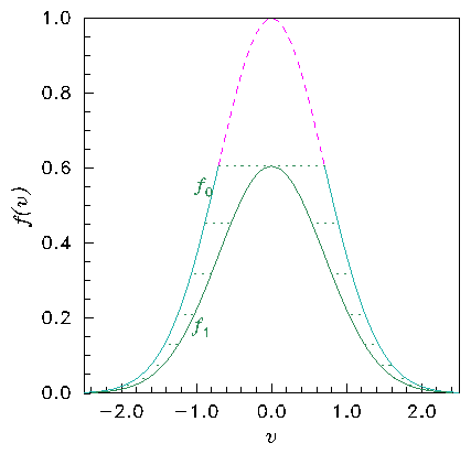
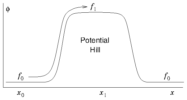
height does not occur at the same <em>velocity</em>. Fig.&nbsp;<a href="chap8.xml#constonorbit">8.5</a> illustrates this fact.

<div class="p"><!----></div>

<div class="p"><!----></div>
<a id="tth_fIg8.5">
</a> <img src="figures/constantorbit.png" alt="figures/constantorbit.png" /><a id="constantorbit">
</a><img src="figures/potentialhill.png" alt="figures/potentialhill.png" /><a id="potentialhill">
</a>


<div style="text-align:center">Figure 8.5: In the collisionless Boltzmann equation the distribution is
  constant along orbits. The distribution (a) is different at the top
  of a potential hill (b) because the speed on an orbit is smaller
  (conserving energy). The distribution values <math xmlns="http://www.w3.org/1998/Math/MathML">
<mrow>
<msub><mrow><mi>f</mi></mrow><mrow><mn>0</mn></mrow>
</msub>
<mo>=</mo><mi>f</mi><mo stretchy="false">(</mo>
<msub><mrow><mi>x</mi></mrow><mrow><mn>0</mn></mrow>
</msub>
<mo stretchy="false">)</mo></mrow></math> and
  <math xmlns="http://www.w3.org/1998/Math/MathML">
<mrow>
<msub><mrow><mi>f</mi></mrow><mrow><mn>1</mn></mrow>
</msub>
<mo>=</mo><mi>f</mi><mo stretchy="false">(</mo>
<msub><mrow><mi>x</mi></mrow><mrow><mn>1</mn></mrow>
</msub>
<mo stretchy="false">)</mo></mrow></math> are the same but at different velocities. Orbits have
  moved the distribution along the horizontal dotted lines in (a). The
  lowest velocity orbits of distribution <math xmlns="http://www.w3.org/1998/Math/MathML">
<mrow>
<msub><mrow><mi>f</mi></mrow><mrow><mn>0</mn></mrow>
</msub>
</mrow></math> (upper dashed part) can't
  reach the top of the hill where <math xmlns="http://www.w3.org/1998/Math/MathML">
<mrow>
<msub><mrow><mi>f</mi></mrow><mrow><mn>1</mn></mrow>
</msub>
</mrow></math> is, and do not contribute to
  it.<a id="constonorbit">
</a></div>

<div class="p"><!----></div>
     <a id="tth_sEc8.3.2"></a><h3>
8.3.2&nbsp;&nbsp;Orbits are Characteristics</h3><a id="characteristicsec">
</a>

<div class="p"><!----></div>
Every hyperbolic partial differential equation can be analysed in a
manner equivalent to the integration along orbits. This approach is
called the method of characteristics<a 
id="characteristic83504"></a>. The
terminology "characteristic"<a 
id="method_of_characteristics83505"></a> is the
general term for what we've called in the context of the Boltzmann
equation an "orbit". Suppose we have a first order linear equation,
an advection equation<a 
id="advection83506"></a> with source<a 
id="source83507"></a>
<a id="hyper1st">
</a><br />
<table width="100%"><tr><td align="center">
    <math xmlns="http://www.w3.org/1998/Math/MathML">
    <mstyle displaystyle="true"><mrow><mi mathvariant="bold">v</mi><mo>.</mo>
<mfrac><mrow><mo>&part;</mo></mrow>
<mrow><mo>&part;</mo><mi mathvariant="bold">x</mi></mrow>
</mfrac>
<mi mathvariant="italic">&psi;</mi><mo>=</mo><mi>S</mi><mo>,</mo></mrow>
    </mstyle></math></td><td width="1">
    <math xmlns="http://www.w3.org/1998/Math/MathML">
    <mstyle displaystyle="true"><mrow><mo stretchy="false">(</mo><mn>8</mn><mo>.</mo><mn>16</mn><mo stretchy="false">)</mo></mrow>
    </mstyle></math>
</td></tr></table>


in which the components of the <math xmlns="http://www.w3.org/1998/Math/MathML">
<mrow><mi>N</mi></mrow></math>-dimensional vector <math xmlns="http://www.w3.org/1998/Math/MathML">
<mrow><mi mathvariant="bold">v</mi></mrow></math> are
simply known functions of <math xmlns="http://www.w3.org/1998/Math/MathML">
<mrow><mi mathvariant="italic">&psi;</mi></mrow></math> and the <math xmlns="http://www.w3.org/1998/Math/MathML">
<mrow><mi>N</mi></mrow></math>-dimensional independent
variables <math xmlns="http://www.w3.org/1998/Math/MathML">
<mrow><mi mathvariant="bold">x</mi></mrow></math>.  Introduce a new parameter <math xmlns="http://www.w3.org/1998/Math/MathML">
<mrow><mi>t</mi></mrow></math> which is going to
serve like time. (If the original equation already contained time as
one of the independent variables, treat it just as one component of
the vector <math xmlns="http://www.w3.org/1998/Math/MathML">
<mrow><mi mathvariant="bold">v</mi></mrow></math> and use the new <math xmlns="http://www.w3.org/1998/Math/MathML">
<mrow><mi>t</mi></mrow></math> as a parameterization.) Think
of the <math xmlns="http://www.w3.org/1998/Math/MathML">
<mrow><mi mathvariant="bold">v</mi></mrow></math> as velocities in <math xmlns="http://www.w3.org/1998/Math/MathML">
<mrow><mi>N</mi></mrow></math>-dimensional space such that
<math xmlns="http://www.w3.org/1998/Math/MathML">
<mrow><mi>d</mi><mi mathvariant="bold">x</mi><mo stretchy="false">/</mo><mi mathvariant="italic">dt</mi><mo>=</mo><mi mathvariant="bold">v</mi></mrow></math>. Remember, in the original formulation, those
<math xmlns="http://www.w3.org/1998/Math/MathML">
<mrow><mi mathvariant="bold">v</mi></mrow></math> were just the coefficients of the partial derivatives in the
respective directions. What we've done is to address the question
"what if the coefficients <math xmlns="http://www.w3.org/1998/Math/MathML">
<mrow><mi mathvariant="bold">v</mi></mrow></math> were velocities?"&nbsp;in respect of
the new <math xmlns="http://www.w3.org/1998/Math/MathML">
<mrow><mi>t</mi></mrow></math> parameter we introduced. The answer is that starting from
any point <math xmlns="http://www.w3.org/1998/Math/MathML">
<mrow><mi mathvariant="bold">x</mi></mrow></math> we would move with the velocity <math xmlns="http://www.w3.org/1998/Math/MathML">
<mrow><mi mathvariant="bold">v</mi></mrow></math> and
thereby trace out an orbit in the <math xmlns="http://www.w3.org/1998/Math/MathML">
<mrow><mi mathvariant="bold">x</mi></mrow></math>-space. This orbit is what
is called the characteristic of the differential equation. As we
follow the characteristic, the equation we would be satisfying would
be
<a id="characode">
</a><br />
<table width="100%"><tr><td align="center">
    <math xmlns="http://www.w3.org/1998/Math/MathML">
    <mstyle displaystyle="true"><mrow><mi mathvariant="bold">v</mi><mo>.</mo>
<mfrac><mrow><mo>&part;</mo></mrow>
<mrow><mo>&part;</mo><mi mathvariant="bold">x</mi></mrow>
</mfrac>
<mi mathvariant="italic">&psi;</mi><mo>=</mo>
<mfrac><mrow><mi>d</mi><mi mathvariant="bold">x</mi></mrow>
<mrow><mi mathvariant="italic">dt</mi></mrow>
</mfrac>
<mo>.</mo>
<mfrac><mrow><mo>&part;</mo></mrow>
<mrow><mo>&part;</mo><mi mathvariant="bold">x</mi></mrow>
</mfrac>
<mi mathvariant="italic">&psi;</mi><mo>=</mo>
<munderover><mo>&sum;</mo><mrow><mi>j</mi><mo>=</mo><mn>1</mn> </mrow>
<mrow><mi>N</mi></mrow></munderover>
<mfrac><mrow><mi>d</mi>
<msub><mrow><mi>x</mi></mrow><mrow><mi>j</mi></mrow>
</msub>
</mrow>
<mrow><mi mathvariant="italic">dt</mi></mrow>
</mfrac>
<mo>.</mo>
<mfrac><mrow><mo>&part;</mo></mrow>
<mrow><mo>&part;</mo>
<msub><mrow><mi>x</mi></mrow><mrow><mi>j</mi></mrow>
</msub>
</mrow>
</mfrac>
<mi mathvariant="italic">&psi;</mi><mo>=</mo>
<msub><mrow><mo> </mo>
<mfrac><mrow><mi>d</mi><mi mathvariant="italic">&psi;</mi></mrow>
<mrow><mi mathvariant="italic">dt</mi></mrow>
</mfrac>
<mo>|</mo></mrow><mrow><mi fontstyle="normal">orbit</mi></mrow>
</msub>
<mo>=</mo><mi>S</mi><mo>.</mo></mrow>
    </mstyle></math></td><td width="1">
    <math xmlns="http://www.w3.org/1998/Math/MathML">
    <mstyle displaystyle="true"><mrow><mo stretchy="false">(</mo><mn>8</mn><mo>.</mo><mn>17</mn><mo stretchy="false">)</mo></mrow>
    </mstyle></math>
</td></tr></table>


This equation is an ordinary differential equation along the
characteristic and can be integrated as <math xmlns="http://www.w3.org/1998/Math/MathML">
<mrow>
<msub><mrow><mi mathvariant="italic">&psi;</mi></mrow><mrow><mn>1</mn></mrow>
</msub>
<mo>-</mo>
<msub><mrow><mi mathvariant="italic">&psi;</mi></mrow><mrow><mn>0</mn></mrow>
</msub>
<mo>=</mo>
<msubsup><mrow><mo>&int;</mo></mrow><mrow><mn>0</mn> </mrow>
<mrow><mn>1</mn></mrow></msubsup>
<mi>S</mi><mi mathvariant="italic">dt</mi></mrow></math>. This process is exactly what we did for Boltzmann's equation. The
only difference is that Boltzmann's equation already contained
time. Fortunately the coefficient of <math xmlns="http://www.w3.org/1998/Math/MathML">
<mrow>
<mfrac><mrow><mo>&part;</mo></mrow>
<mrow><mo>&part;</mo><mi>t</mi></mrow>
</mfrac>
</mrow></math> in
Boltzmann's equation is 1. Therefore it was possible to choose the
time-like parameter to be actual physical time, which we did.  We
could however have made a different choice, if we'd preferred.  We
also used notation familiar from fluid theory for the "convective"
derivative <math xmlns="http://www.w3.org/1998/Math/MathML">
<mrow><mi>D</mi><mo stretchy="false">/</mo><mi mathvariant="italic">Dt</mi></mrow></math>, but that is no different from <math xmlns="http://www.w3.org/1998/Math/MathML">
<mrow><mi>d</mi><mo stretchy="false">/</mo><mi mathvariant="italic">dt</mi></mrow></math> along the
orbit.

<div class="p"><!----></div>
Higher order scalar equations can be rendered into first order,
<em>vector</em> (multiple dependent variable) equations, as we saw
before. If they are hyperbolic, then they have characteristics which
correspond to the coefficients of the eigenvectors of the
equations. Those eigenvectors must be real<a 
id="eigenvalue_real83508"></a>
otherwise the presumption that there are real characteristics breaks
down. The condition, therefore, for a system of vector equations to be
hyperbolic<a 
id="hyperbolic83509"></a> is that they are diagonalizable with real
eigenvectors.

<div class="p"><!----></div>
 <a id="tth_sEc8.4"></a><h2>
8.4&nbsp;&nbsp;Collision Term</h2>

<div class="p"><!----></div>
<a 
id="collision84510"></a>The importance of the Boltzmann equation's collision term depends upon the
application. In some plasma and gravitational applications it can be
completely neglected and ignored. Collisions are nothing.  Then the
equation of interest is called the Vlasov equation<a 
id="Vlasov_equation84511"></a>.
<a id="Vlasov">
</a><br />
<table width="100%"><tr><td align="center">
    <math xmlns="http://www.w3.org/1998/Math/MathML">
    <mstyle displaystyle="true"><mrow>
<mfrac><mrow><mo>&part;</mo><mi>f</mi></mrow>
<mrow><mo>&part;</mo><mi>t</mi></mrow>
</mfrac>
<mo>+</mo><mi mathvariant="bold-italic">v</mi><mo>.</mo>
<mfrac><mrow><mo>&part;</mo><mi>f</mi></mrow>
<mrow><mo>&part;</mo><mi mathvariant="bold-italic">x</mi></mrow>
</mfrac>
<mo>+</mo><mi mathvariant="bold-italic">a</mi><mo>.</mo>
<mfrac><mrow><mo>&part;</mo><mi>f</mi></mrow>
<mrow><mo>&part;</mo><mi mathvariant="bold-italic">v</mi></mrow>
</mfrac>
<mo>=</mo><mn>0</mn><mo>.</mo></mrow>
    </mstyle></math></td><td width="1">
    <math xmlns="http://www.w3.org/1998/Math/MathML">
    <mstyle displaystyle="true"><mrow><mo stretchy="false">(</mo><mn>8</mn><mo>.</mo><mn>18</mn><mo stretchy="false">)</mo></mrow>
    </mstyle></math>
</td></tr></table>


At the other extreme, when applied forces are negligible so <math xmlns="http://www.w3.org/1998/Math/MathML">
<mrow><mi mathvariant="bold-italic">a</mi><mo>=</mo><mn>0</mn></mrow></math>,
and the problem is homogeneous and steady state
<math xmlns="http://www.w3.org/1998/Math/MathML">
<mrow><mo>&part;</mo><mo stretchy="false">/</mo><mo>&part;</mo><mi mathvariant="bold-italic">x</mi><mo>=</mo><mn>0</mn></mrow></math>, <math xmlns="http://www.w3.org/1998/Math/MathML">
<mrow><mo>&part;</mo><mo stretchy="false">/</mo><mo>&part;</mo><mi>t</mi><mo>=</mo><mn>0</mn></mrow></math>, all that is
left of the Boltzmann equation is <math xmlns="http://www.w3.org/1998/Math/MathML">
<mrow><mi>C</mi><mo>=</mo><mn>0</mn></mrow></math>. So then collisions are everything!

<div class="p"><!----></div>
Also, the form of the collision term depends upon
application. Especially it depends upon whether the important
collisions are with the same particles or with some particles of a
different type that are described by a different distribution
function. 

<div class="p"><!----></div>
     <a id="tth_sEc8.4.1"></a><h3>
8.4.1&nbsp;&nbsp;Self-scattering</h3>

<div class="p"><!----></div>
<a 
id="scattering84512"></a><a 
id="self-scattering84513"></a> Self-scattering dominates, for example, a
simple unreactive monatomic gas.  There is just one species of
particle. And elastic<a 
id="elastic_scattering84514"></a> self-scattering is the
only type of collision present. Then the integrals over all velocity
space of <math xmlns="http://www.w3.org/1998/Math/MathML">
<mrow><mi>C</mi></mrow></math>, <math xmlns="http://www.w3.org/1998/Math/MathML">
<mrow><mi mathvariant="bold-italic">v</mi><mi>C</mi></mrow></math>, and <math xmlns="http://www.w3.org/1998/Math/MathML">
<mrow>
<msup><mrow><mi mathvariant="bold-italic">v</mi></mrow><mrow><mn>2</mn></mrow>
</msup>
<mi>C</mi></mrow></math> are zero. That is a simple
consequence of particle, momentum, and energy conservation.  With
self-scattering, though, other complications are severe. The rate at
which collisions take place depends upon a product
<math xmlns="http://www.w3.org/1998/Math/MathML">
<mrow><mi>f</mi><mo stretchy="false">(</mo>
<msub><mrow><mi mathvariant="bold-italic">v</mi></mrow><mrow><mn>1</mn></mrow>
</msub>
<mo stretchy="false">)</mo><mi>f</mi><mo stretchy="false">(</mo>
<msub><mrow><mi mathvariant="bold-italic">v</mi></mrow><mrow><mn>2</mn></mrow>
</msub>
<mo stretchy="false">)</mo></mrow></math> of the distribution functions of the two
colliding particles of different velocities (so it is non-linear). It
is multiplied by the collision rate, which is the cross-section (a
function of relative speed) times the relative speed
<math xmlns="http://www.w3.org/1998/Math/MathML">
<mrow><mi mathvariant="italic">&sigma;</mi><mo stretchy="false">&verbar;</mo>
<msub><mrow><mi mathvariant="bold-italic">v</mi></mrow><mrow><mn>1</mn></mrow>
</msub>
<mo>-</mo>
<msub><mrow><mi mathvariant="bold-italic">v</mi></mrow><mrow><mn>2</mn></mrow>
</msub>
<mo stretchy="false">&verbar;</mo></mrow></math>. It is then integrated over the velocity
<math xmlns="http://www.w3.org/1998/Math/MathML">
<mrow>
<msub><mrow><mi mathvariant="bold-italic">v</mi></mrow><mrow><mn>2</mn></mrow>
</msub>
</mrow></math> of the target particle (so Boltzmann's equation becomes an
integro-differential equation<a 
id="integro-differential84515"></a>). Generally
substantial approximation is necessary to make the collision term
managable, even for numerical solution.

<div class="p"><!----></div>
     <a id="tth_sEc8.4.2"></a><h3>
8.4.2&nbsp;&nbsp;No self-scattering</h3>

<div class="p"><!----></div>
If, however, the dominant interactions are with a different type of
particle, then momentum and energy of the first species is not
necessarily conserved. It can be transferred to the second
species. But at least<a 
id="linear_collision_term84516"></a> the collision term
is linear in <math xmlns="http://www.w3.org/1998/Math/MathML">
<mrow><mi>f</mi></mrow></math>, and if the initial velocity distribution of the
second species is known or may be neglected, then substantial
reduction of the need for integration can occur.

<div class="p"><!----></div>
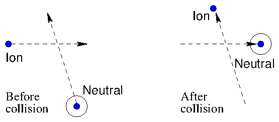
For example, as illustrated in Fig.&nbsp;<a href="chap8.xml#lBGKcoln">8.6</a>, a form of
collision term that approximately represents
charge-exchange<a 
id="charge-exchange84517"></a> collisions at a fixed rate
<math xmlns="http://www.w3.org/1998/Math/MathML">
<mrow><mi mathvariant="italic">&nu;</mi></mrow></math> between singly charged ions (the species whose Boltzman equation we
are trying to solve) and neutrals of the same element (the target
species 2) is
<a id="BGKcoln">
</a><br />
<table width="100%"><tr><td align="center">
    <math xmlns="http://www.w3.org/1998/Math/MathML">
    <mstyle displaystyle="true"><mrow><mi>C</mi><mo stretchy="false">(</mo><mi>f</mi><mo stretchy="false">)</mo><mo>=</mo><mo>-</mo><mi mathvariant="italic">&nu;</mi><mi>f</mi><mo stretchy="false">(</mo><mi mathvariant="bold-italic">v</mi><mo stretchy="false">)</mo><mo>+</mo><mi mathvariant="italic">&nu;</mi>
<msub><mrow><mi>f</mi></mrow><mrow><mn>2</mn></mrow>
</msub>
<mo stretchy="false">(</mo><mi mathvariant="bold-italic">v</mi><mo stretchy="false">)</mo><mo>.</mo></mrow>
    </mstyle></math></td><td width="1">
    <math xmlns="http://www.w3.org/1998/Math/MathML">
    <mstyle displaystyle="true"><mrow><mo stretchy="false">(</mo><mn>8</mn><mo>.</mo><mn>19</mn><mo stretchy="false">)</mo></mrow>
    </mstyle></math>
</td></tr></table>


<div class="p"><!----></div>
<a id="tth_fIg8.6">
</a>   <img src="figures/chargeexch.png" alt="figures/chargeexch.png" /><a id="chargeexch">
</a>
  
<div style="text-align:center">Figure 8.6: Charge exchange collisions, where an electron is
    transferred from a neutral to an ion, give rise to a simple
    collision term. If they occur at a constant rate, <math xmlns="http://www.w3.org/1998/Math/MathML">
<mrow><mi mathvariant="italic">&nu;</mi></mrow></math>, eq.&nbsp;    <a href="chap8.xml#BGKcoln">8.19</a> applies.<a id="lBGKcoln">
</a></div>

<div class="p"><!----></div>
This is sometimes called the BGK<a 
id="BGK_collision_term84518"></a> collision
form. It represents depletion of the original ions at rate <math xmlns="http://www.w3.org/1998/Math/MathML">
<mrow><mi mathvariant="italic">&nu;</mi></mrow></math>
giving the term <math xmlns="http://www.w3.org/1998/Math/MathML">
<mrow><mo>-</mo><mi mathvariant="italic">&nu;</mi><mi>f</mi><mo stretchy="false">(</mo><mi mathvariant="bold-italic">v</mi><mo stretchy="false">)</mo></mrow></math>, and their direct replacement at the same
rate by new ions.  The newly born ions, before their collision, were
neutrals. They retain the velocity distribution <math xmlns="http://www.w3.org/1998/Math/MathML">
<mrow>
<msub><mrow><mi>f</mi></mrow><mrow><mn>2</mn></mrow>
</msub>
<mo stretchy="false">(</mo><mi mathvariant="bold-italic">v</mi><mo stretchy="false">)</mo></mrow></math> they had
before the collision, because the collision just transfers an electron
from one to the other.

<div class="p"><!----></div>
Another idealized example (Fig.&nbsp;<a href="chap8.xml#lisotropic">8.7</a>) is when collisions
are with heavy stationary targets<a 
id="stationary_targets84519"></a> (which
therefore acquire negligible recoil energy) which happen to scatter equally,
isotropically, in all directions.
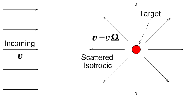
<div class="p"><!----></div>
<a id="tth_fIg8.7">
</a>   <img src="figures/isotropscat.png" alt="figures/isotropscat.png" /><a id="isotropscat">
</a>
  
<div style="text-align:center">Figure 8.7: Isotropic scattering (an idealized approximation) gives
    particles emerging equally in all directions <math xmlns="http://www.w3.org/1998/Math/MathML">
<mrow><mi mathvariant="italic">&Omega;</mi></mrow></math>. With heavy
    targets, <math xmlns="http://www.w3.org/1998/Math/MathML">
<mrow><mi>v</mi></mrow></math> is not changed in magnitude, only in direction. Eq.&nbsp;    (<a href="chap8.xml#isotropic">8.20</a>) is the result.<a id="lisotropic">
</a></div>

<div class="p"><!----></div>
In a collision, a particle
just changes the direction of its velocity, not its magnitude.
If the density of targets is <math xmlns="http://www.w3.org/1998/Math/MathML">
<mrow>
<msub><mrow><mi>n</mi></mrow><mrow><mn>2</mn></mrow>
</msub>
</mrow></math> and the collision cross-section is
<math xmlns="http://www.w3.org/1998/Math/MathML">
<mrow><mi mathvariant="italic">&sigma;</mi></mrow></math>, then
<a id="isotropic">
</a><br />
<table width="100%"><tr><td align="center">
    <math xmlns="http://www.w3.org/1998/Math/MathML">
    <mstyle displaystyle="true"><mrow><mi>C</mi><mo stretchy="false">(</mo><mi>f</mi><mo stretchy="false">)</mo><mo>=</mo><mo>-</mo>
<msub><mrow><mi>n</mi></mrow><mrow><mn>2</mn></mrow>
</msub>
<mi mathvariant="italic">&sigma;</mi><mi>v</mi><mrow><mo>(</mo><mi>f</mi><mo stretchy="false">(</mo><mi mathvariant="bold-italic">v</mi><mo stretchy="false">)</mo><mo>-</mo><mo>&int;</mo><mi>f</mi><mo stretchy="false">(</mo><mi mathvariant="bold-italic">v</mi><mo stretchy="false">)</mo>
<msup><mrow><mi>d</mi></mrow><mrow><mn>2</mn></mrow>
</msup>
<mi mathvariant="italic">&Omega;</mi><mo stretchy="false">/</mo><mn>4</mn><mi mathvariant="italic">&pi;</mi><mo>)</mo></mrow><mo>.</mo></mrow>
    </mstyle></math></td><td width="1">
    <math xmlns="http://www.w3.org/1998/Math/MathML">
    <mstyle displaystyle="true"><mrow><mo stretchy="false">(</mo><mn>8</mn><mo>.</mo><mn>20</mn><mo stretchy="false">)</mo></mrow>
    </mstyle></math>
</td></tr></table>


Here<a 
id="solid_angle___Omega_84520"></a> <math xmlns="http://www.w3.org/1998/Math/MathML">
<mrow>
<msup><mrow><mi>d</mi></mrow><mrow><mn>2</mn></mrow>
</msup>
<mi mathvariant="italic">&Omega;</mi><mo>=</mo><mi>sin</mi><mi mathvariant="italic">&theta;</mi><mi>d</mi><mi mathvariant="italic">&theta;</mi><mi>d</mi><mi mathvariant="italic">&chi;</mi></mrow></math> is the
element of solid angle, and the integral is over the angular position
(<math xmlns="http://www.w3.org/1998/Math/MathML">
<mrow><mi mathvariant="italic">&theta;</mi><mo>,</mo><mi mathvariant="italic">&chi;</mi></mrow></math>) on the surface of the sphere in velocity space at
constant total velocity <math xmlns="http://www.w3.org/1998/Math/MathML">
<mrow><mi>v</mi></mrow></math>. In other words, the second term is the
average of the distribution function over all directions, at <math xmlns="http://www.w3.org/1998/Math/MathML">
<mrow><mi>v</mi></mrow></math>. This
type of collision scatters the velocity direction, thus tending to
remove any anisotropy (variation with angles <math xmlns="http://www.w3.org/1998/Math/MathML">
<mrow><mi mathvariant="italic">&theta;</mi></mrow></math> or <math xmlns="http://www.w3.org/1998/Math/MathML">
<mrow><mi mathvariant="italic">&chi;</mi></mrow></math>.)

<div class="p"><!----></div>
It should be noticed that in these examples where self-collisions can
be ignored, the collision term generally consists of two parts. The
first is negative, the removal or "sink"<a 
id="sink_of_particles84521"></a>
rate of particles that collide with whatever targets happen to be
present (<math xmlns="http://www.w3.org/1998/Math/MathML">
<mrow><mo>-</mo>
<msub><mrow><mi>n</mi></mrow><mrow><mn>2</mn></mrow>
</msub>
<mi mathvariant="italic">&sigma;</mi><mi>v</mi><mi>f</mi></mrow></math> in eq.<a href="chap8.xml#isotropic">8.20</a>). The second is
positive, the "source"<a 
id="source_of_particles84522"></a> rate of particles
from all mechanisms. When non-reactive gases are being treated, the
source is only the re-emergence of particles from collisions. But in
other situations, such as neutron transport in a reactor, generation
of new particles from reactions or spontaneous emission from the
target medium may be equally important.

<div class="p"><!----></div>
For multiple target species, <math xmlns="http://www.w3.org/1998/Math/MathML">
<mrow><mi>j</mi></mrow></math>, the sink term is the sum of collisions
with all target types. And this is often written in shorthand as
<math xmlns="http://www.w3.org/1998/Math/MathML">
<mrow><mo>-</mo>
<msub><mrow><mi mathvariant="italic">&Sigma;</mi></mrow><mrow><mi>t</mi></mrow>
</msub>
<mo>&times;</mo><mo stretchy="false">(</mo><mi>v</mi><mi>f</mi><mo stretchy="false">)</mo></mrow></math>, with
<a id="macrocross">
</a><br />
<table width="100%"><tr><td align="center">
    <math xmlns="http://www.w3.org/1998/Math/MathML">
    <mstyle displaystyle="true"><mrow>
<msub><mrow><mi mathvariant="italic">&Sigma;</mi></mrow><mrow><mi>t</mi></mrow>
</msub>
<mo>=</mo>
<munder><mo>&sum;</mo><mrow><mi>j</mi></mrow>
</munder>

<msub><mrow><mi>n</mi></mrow><mrow><mi>j</mi></mrow>
</msub>

<msub><mrow><mi mathvariant="italic">&sigma;</mi></mrow><mrow><mi>j</mi></mrow>
</msub>
<mo>;</mo></mrow>
    </mstyle></math></td><td width="1">
    <math xmlns="http://www.w3.org/1998/Math/MathML">
    <mstyle displaystyle="true"><mrow><mo stretchy="false">(</mo><mn>8</mn><mo>.</mo><mn>21</mn><mo stretchy="false">)</mo></mrow>
    </mstyle></math>
</td></tr></table>


and referred to in reactor physics literature as the "macroscopic
cross-section"<a 
id="macroscopic_cross-section84523"></a>. This terminology is
unfortunate because the quantity <math xmlns="http://www.w3.org/1998/Math/MathML">
<mrow>
<msub><mrow><mi mathvariant="italic">&Sigma;</mi></mrow><mrow><mi>t</mi></mrow>
</msub>
</mrow></math> has units m<math xmlns="http://www.w3.org/1998/Math/MathML">
<mrow>
<msup><mrow></mrow><mrow><mo>-</mo><mn>1</mn></mrow>
</msup>
</mrow></math> not
m<math xmlns="http://www.w3.org/1998/Math/MathML">
<mrow>
<msup><mrow></mrow><mrow><mn>2</mn></mrow>
</msup>
</mrow></math>, and is an inverse attenuation-length<a 
id="attenuation-length84524"></a>,
not a cross section. When the targets are stationary, <math xmlns="http://www.w3.org/1998/Math/MathML">
<mrow>
<msub><mrow><mi mathvariant="italic">&Sigma;</mi></mrow><mrow><mi>t</mi></mrow>
</msub>
</mrow></math> is
isotropic: the rate of collisions is independent of the direction of
particle velocity. The source term, by contrast, is <em>not</em> usually isotropic
because it includes the emergence of particles from pure scattering
events. Scattering, even from stationary targets, usually partially
retains any anisotropy in the distribution function itself. (The
conditions of eq.&nbsp;<a href="chap8.xml#isotropic">8.20</a> are a non-typical idealization.)

<div class="p"><!----></div>

<h2>Worked Example: Solving Vlasov's Equation</h2>

<div class="p"><!----></div>
Consider<a 
id="Vlasov_equation84525"></a> a steady-state situation, one
dimensional in space and velocity, where acceleration arises only from
a spatially varying potential energy of the form <math xmlns="http://www.w3.org/1998/Math/MathML">
<mrow><mi mathvariant="italic">&phi;</mi><mo stretchy="false">(</mo><mi>x</mi><mo stretchy="false">)</mo><mo>=</mo>
<msub><mrow><mi mathvariant="italic">&phi;</mi></mrow><mrow><mn>0</mn></mrow>
</msub>
<mi>exp</mi><mo stretchy="false">(</mo><mo>-</mo>
<msup><mrow><mi>x</mi></mrow><mrow><mn>2</mn></mrow>
</msup>
<mo stretchy="false">/</mo>
<msup><mrow><mi>w</mi></mrow><mrow><mn>2</mn></mrow>
</msup>
<mo stretchy="false">)</mo></mrow></math>, so <math xmlns="http://www.w3.org/1998/Math/MathML">
<mrow><mi>a</mi><mo>=</mo><mo>-</mo>
<mfrac><mrow><mn>1</mn></mrow>
<mrow><mi>m</mi></mrow>
</mfrac>
<mi>d</mi><mi mathvariant="italic">&phi;</mi><mo stretchy="false">/</mo><mi mathvariant="italic">dx</mi></mrow></math>, and collisions are
negligible. If the distribution function at <math xmlns="http://www.w3.org/1998/Math/MathML">
<mrow><mo stretchy="false">&verbar;</mo><mi>x</mi><mo stretchy="false">&verbar;</mo><mo>&rarr;</mo><mi mathvariant="italic">&infin;</mi></mrow></math> is equal
to <math xmlns="http://www.w3.org/1998/Math/MathML">
<mrow>
<msub><mrow><mi>f</mi></mrow><mrow><mi mathvariant="italic">&infin;</mi></mrow>
</msub>
<mo stretchy="false">(</mo><mi>v</mi><mo stretchy="false">)</mo><mo>=</mo><mi>exp</mi><mo stretchy="false">(</mo><mo>-</mo><mi>m</mi>
<msup><mrow><mi>v</mi></mrow><mrow><mn>2</mn></mrow>
</msup>
<mo stretchy="false">/</mo><mn>2</mn><mi>T</mi><mo stretchy="false">)</mo></mrow></math>, and <math xmlns="http://www.w3.org/1998/Math/MathML">
<mrow>
<msub><mrow><mi mathvariant="italic">&phi;</mi></mrow><mrow><mn>0</mn></mrow>
</msub>
<mo>&ge;</mo><mn>0</mn></mrow></math>, find the
distribution function <math xmlns="http://www.w3.org/1998/Math/MathML">
<mrow><mi>f</mi><mo stretchy="false">(</mo><mi>v</mi><mo>,</mo><mi>x</mi><mo stretchy="false">)</mo></mrow></math> for all <math xmlns="http://www.w3.org/1998/Math/MathML">
<mrow><mi>x</mi></mrow></math>, and <math xmlns="http://www.w3.org/1998/Math/MathML">
<mrow><mi>v</mi></mrow></math>. Can you solve
this problem if <math xmlns="http://www.w3.org/1998/Math/MathML">
<mrow>
<msub><mrow><mi mathvariant="italic">&phi;</mi></mrow><mrow><mn>0</mn></mrow>
</msub>
<mo>&lt;</mo><mn>0</mn></mrow></math>?
<div class="p"><!----></div>
<br />The steady collisionless one-dimensional Boltzmann (Vlasov) equation
is<a 
id="steady_state84526"></a>
<br />
<table width="100%"><tr><td align="center">
    <math xmlns="http://www.w3.org/1998/Math/MathML">
    <mstyle displaystyle="true"><mrow><mn>0</mn><mo>=</mo>
<mfrac><mrow><mi>D</mi><mi>f</mi></mrow>
<mrow><mi>D</mi><mi>t</mi></mrow>
</mfrac>
<mo>=</mo><mi>v</mi><mo>.</mo>
<mfrac><mrow><mo>&part;</mo><mi>f</mi></mrow>
<mrow><mo>&part;</mo><mi>x</mi></mrow>
</mfrac>
<mo>+</mo><mi>a</mi><mo>.</mo>
<mfrac><mrow><mo>&part;</mo><mi>f</mi></mrow>
<mrow><mo>&part;</mo><mi>v</mi></mrow>
</mfrac>
</mrow>
    </mstyle></math></td><td width="1">
    <math xmlns="http://www.w3.org/1998/Math/MathML">
    <mstyle displaystyle="true"><mrow><mo stretchy="false">(</mo><mn>8</mn><mo>.</mo><mn>22</mn><mo stretchy="false">)</mo></mrow>
    </mstyle></math>
</td></tr></table>


The equations of the orbit (the characteristics)
are<a 
id="characteristic_equation84527"></a>
<br />
<table width="100%"><tr><td align="center">
    <math xmlns="http://www.w3.org/1998/Math/MathML">
    <mstyle displaystyle="true"><mrow>
<mfrac><mrow><mi>d</mi><mi>x</mi></mrow>
<mrow><mi>d</mi><mi>t</mi></mrow>
</mfrac>
<mo>=</mo><mi>v</mi><mo>;</mo><mi>&emsp;&emsp;&emsp;&emsp;&emsp;&emsp;</mi>
<mfrac><mrow><mi>d</mi><mi>v</mi></mrow>
<mrow><mi>d</mi><mi>t</mi></mrow>
</mfrac>
<mo>=</mo><mi>a</mi><mo>=</mo><mo>-</mo>
<mfrac><mrow><mn>1</mn></mrow>
<mrow><mi>m</mi></mrow>
</mfrac>

<mfrac><mrow><mi>d</mi><mi mathvariant="italic">&phi;</mi></mrow>
<mrow><mi>d</mi><mi>x</mi></mrow>
</mfrac>
<mo>.</mo></mrow>
    </mstyle></math></td><td width="1">
    <math xmlns="http://www.w3.org/1998/Math/MathML">
    <mstyle displaystyle="true"><mrow><mo stretchy="false">(</mo><mn>8</mn><mo>.</mo><mn>23</mn><mo stretchy="false">)</mo></mrow>
    </mstyle></math>
</td></tr></table>


Multiplying the second of these by the first we find
<br />
<table width="100%"><tr><td align="center">
    <math xmlns="http://www.w3.org/1998/Math/MathML">
    <mstyle displaystyle="true"><mrow><mi>v</mi>
<mfrac><mrow><mi>d</mi><mi>v</mi></mrow>
<mrow><mi>d</mi><mi>t</mi></mrow>
</mfrac>
<mo>+</mo>
<mfrac><mrow><mn>1</mn></mrow>
<mrow><mi>m</mi></mrow>
</mfrac>

<mfrac><mrow><mi>d</mi><mi mathvariant="italic">&phi;</mi></mrow>
<mrow><mi>d</mi><mi>x</mi></mrow>
</mfrac>

<mfrac><mrow><mi>d</mi><mi>x</mi></mrow>
<mrow><mi>d</mi><mi>t</mi></mrow>
</mfrac>
<mo>=</mo><mn>0</mn><mo>,</mo></mrow>
    </mstyle></math></td><td width="1">
    <math xmlns="http://www.w3.org/1998/Math/MathML">
    <mstyle displaystyle="true"><mrow><mo stretchy="false">(</mo><mn>8</mn><mo>.</mo><mn>24</mn><mo stretchy="false">)</mo></mrow>
    </mstyle></math>
</td></tr></table>


which may be immediately integrated to find
<br />
<table width="100%"><tr><td align="center">
    <math xmlns="http://www.w3.org/1998/Math/MathML">
    <mstyle displaystyle="true"><mrow>
<mfrac><mrow><mn>1</mn></mrow>
<mrow><mn>2</mn></mrow>
</mfrac>
<mi>m</mi>
<msup><mrow><mi>v</mi></mrow><mrow><mn>2</mn></mrow>
</msup>
<mo>+</mo><mi mathvariant="italic">&phi;</mi><mo>=</mo><mi mathvariant="italic">const</mi><mo>.</mo></mrow>
    </mstyle></math></td><td width="1">
    <math xmlns="http://www.w3.org/1998/Math/MathML">
    <mstyle displaystyle="true"><mrow><mo stretchy="false">(</mo><mn>8</mn><mo>.</mo><mn>25</mn><mo stretchy="false">)</mo></mrow>
    </mstyle></math>
</td></tr></table>


We have derived the conservation of energy, kinetic plus
potential. The constant can be considered to be the kinetic energy at
infinity, <math xmlns="http://www.w3.org/1998/Math/MathML">
<mrow>
<mfrac><mrow><mn>1</mn></mrow>
<mrow><mn>2</mn></mrow>
</mfrac>

<msubsup><mrow><mi mathvariant="italic">mv</mi></mrow><mrow><mi mathvariant="italic">&infin;</mi> </mrow>
<mrow><mn>2</mn></mrow></msubsup>
</mrow></math>, where the potential (<math xmlns="http://www.w3.org/1998/Math/MathML">
<mrow>
<msub><mrow><mi mathvariant="italic">&phi;</mi></mrow><mrow><mi mathvariant="italic">&infin;</mi></mrow>
</msub>
</mrow></math>) is zero. 

<div class="p"><!----></div>
For Vlasov's equation, the distribution function, <math xmlns="http://www.w3.org/1998/Math/MathML">
<mrow><mi>f</mi></mrow></math> is constant
along the orbits<a 
id="constant_along_orbit84528"></a>. Therefore
<br />
<table width="100%"><tr><td align="center">
    <math xmlns="http://www.w3.org/1998/Math/MathML">
    <mstyle displaystyle="true"><mrow><mi>f</mi><mo stretchy="false">(</mo><mi>v</mi><mo>,</mo><mi>x</mi><mo stretchy="false">)</mo><mo>=</mo>
<msub><mrow><mi>f</mi></mrow><mrow><mi mathvariant="italic">&infin;</mi></mrow>
</msub>
<mo stretchy="false">(</mo>
<msub><mrow><mi>v</mi></mrow><mrow><mi mathvariant="italic">&infin;</mi></mrow>
</msub>
<mo stretchy="false">)</mo><mo>=</mo><mi>exp</mi><mo stretchy="false">(</mo><mo>-</mo><mi>m</mi>
<msubsup><mrow><mi>v</mi></mrow><mrow><mi mathvariant="italic">&infin;</mi> </mrow>
<mrow><mn>2</mn></mrow></msubsup>
<mo stretchy="false">/</mo><mn>2</mn><mi>T</mi><mo stretchy="false">)</mo><mo>=</mo><mi>exp</mi><mo stretchy="false">(</mo><mo>-</mo><mo stretchy="false">[</mo><mi>m</mi>
<msup><mrow><mi>v</mi></mrow><mrow><mn>2</mn></mrow>
</msup>
<mo>+</mo><mn>2</mn><mi mathvariant="italic">&phi;</mi><mo stretchy="false">(</mo><mi>x</mi><mo stretchy="false">)</mo><mo stretchy="false">]</mo><mo stretchy="false">/</mo><mn>2</mn><mi>T</mi><mo stretchy="false">)</mo><mo>.</mo></mrow>
    </mstyle></math></td><td width="1">
    <math xmlns="http://www.w3.org/1998/Math/MathML">
    <mstyle displaystyle="true"><mrow><mo stretchy="false">(</mo><mn>8</mn><mo>.</mo><mn>26</mn><mo stretchy="false">)</mo></mrow>
    </mstyle></math>
</td></tr></table>


Substituting for <math xmlns="http://www.w3.org/1998/Math/MathML">
<mrow><mi mathvariant="italic">&phi;</mi><mo stretchy="false">(</mo><mi>x</mi><mo stretchy="false">)</mo></mrow></math> we find
<br />
<table width="100%"><tr><td align="center">
    <math xmlns="http://www.w3.org/1998/Math/MathML">
    <mstyle displaystyle="true"><mrow><mi>f</mi><mo stretchy="false">(</mo><mi>v</mi><mo>,</mo><mi>x</mi><mo stretchy="false">)</mo><mo>=</mo><mi>exp</mi><mo stretchy="false">(</mo><mo>-</mo><mo stretchy="false">[</mo><mi>m</mi>
<msup><mrow><mi>v</mi></mrow><mrow><mn>2</mn></mrow>
</msup>
<mo>+</mo><mn>2</mn>
<msub><mrow><mi mathvariant="italic">&phi;</mi></mrow><mrow><mn>0</mn></mrow>
</msub>

<msup><mrow><mi>e</mi></mrow><mrow><mo>-</mo>
<msup><mrow><mi>x</mi></mrow><mrow><mn>2</mn></mrow>
</msup>
<mo stretchy="false">/</mo>
<msup><mrow><mi>w</mi></mrow><mrow><mn>2</mn></mrow>
</msup>
</mrow>
</msup>
<mo stretchy="false">]</mo><mo stretchy="false">/</mo><mn>2</mn><mi>T</mi><mo stretchy="false">)</mo><mo>=</mo><mi>exp</mi><mo stretchy="false">(</mo><mo>-</mo>
<mfrac><mrow><mi>m</mi>
<msup><mrow><mi>v</mi></mrow><mrow><mn>2</mn></mrow>
</msup>
</mrow>
<mrow><mn>2</mn><mi>T</mi></mrow>
</mfrac>
<mo stretchy="false">)</mo><mi>exp</mi><mo stretchy="false">(</mo><mo>-</mo>
<mfrac><mrow>
<msub><mrow><mi mathvariant="italic">&phi;</mi></mrow><mrow><mn>0</mn></mrow>
</msub>
</mrow>
<mrow><mi>T</mi></mrow>
</mfrac>

<msup><mrow><mi>e</mi></mrow><mrow><mo>-</mo>
<msup><mrow><mi>x</mi></mrow><mrow><mn>2</mn></mrow>
</msup>
<mo stretchy="false">/</mo>
<msup><mrow><mi>w</mi></mrow><mrow><mn>2</mn></mrow>
</msup>
</mrow>
</msup>
<mo stretchy="false">)</mo><mo>.</mo></mrow>
    </mstyle></math></td><td width="1">
    <math xmlns="http://www.w3.org/1998/Math/MathML">
    <mstyle displaystyle="true"><mrow><mo stretchy="false">(</mo><mn>8</mn><mo>.</mo><mn>27</mn><mo stretchy="false">)</mo></mrow>
    </mstyle></math>
</td></tr></table>


If <math xmlns="http://www.w3.org/1998/Math/MathML">
<mrow>
<msub><mrow><mi mathvariant="italic">&phi;</mi></mrow><mrow><mn>0</mn></mrow>
</msub>
<mo>&gt;</mo><mn>0</mn></mrow></math>, then no matter how small <math xmlns="http://www.w3.org/1998/Math/MathML">
<mrow>
<msup><mrow><mi>v</mi></mrow><mrow><mn>2</mn></mrow>
</msup>
</mrow></math> is, there is a real
solution for <math xmlns="http://www.w3.org/1998/Math/MathML">
<mrow>
<msub><mrow><mi>v</mi></mrow><mrow><mi mathvariant="italic">&infin;</mi></mrow>
</msub>
</mrow></math> to the conservation equation <math xmlns="http://www.w3.org/1998/Math/MathML">
<mrow>
<mfrac><mrow><mn>1</mn></mrow>
<mrow><mn>2</mn></mrow>
</mfrac>
<mi>m</mi>
<msup><mrow><mi>v</mi></mrow><mrow><mn>2</mn></mrow>
</msup>
<mo>+</mo><mi mathvariant="italic">&phi;</mi><mo>=</mo>
<mfrac><mrow><mn>1</mn></mrow>
<mrow><mn>2</mn></mrow>
</mfrac>
<mi>m</mi>
<msubsup><mrow><mi>v</mi></mrow><mrow><mi mathvariant="italic">&infin;</mi> </mrow>
<mrow><mn>2</mn></mrow></msubsup>
</mrow></math>. Therefore this expression for <math xmlns="http://www.w3.org/1998/Math/MathML">
<mrow><mi>f</mi></mrow></math>
is valid for all <math xmlns="http://www.w3.org/1998/Math/MathML">
<mrow><mi>v</mi></mrow></math>. The distribution is everywhere Maxwellian, but
its density varies with position. However, if <math xmlns="http://www.w3.org/1998/Math/MathML">
<mrow>
<msub><mrow><mi mathvariant="italic">&phi;</mi></mrow><mrow><mn>0</mn></mrow>
</msub>
<mo>&lt;</mo><mn>0</mn></mrow></math> then,
everywhere that <math xmlns="http://www.w3.org/1998/Math/MathML">
<mrow><mi mathvariant="italic">&phi;</mi></mrow></math> is negative, there is a minimum speed
<math xmlns="http://www.w3.org/1998/Math/MathML">
<mrow><msqrt><mrow><mo>-</mo><mn>2</mn><mi mathvariant="italic">&phi;</mi><mo stretchy="false">/</mo><mi>m</mi></mrow></msqrt></mrow></math>, below which there is no real solution for
<math xmlns="http://www.w3.org/1998/Math/MathML">
<mrow>
<msub><mrow><mi>v</mi></mrow><mrow><mi mathvariant="italic">&infin;</mi></mrow>
</msub>
</mrow></math>. These are the trapped orbits<a 
id="trapped_orbit84529"></a>. They do
not extend to infinity, but are reflected because they reside in the
potential well. The value of <math xmlns="http://www.w3.org/1998/Math/MathML">
<mrow><mi>f</mi></mrow></math> on those trapped orbits is undefined
by the boundary condition at infinity, and must be determined
otherwise, e.g.&nbsp;from the initial conditions. Fig.&nbsp;<a href="chap8.xml#xhole">8.8</a> shows
an example solution. 

<div class="p"><!----></div>
<a id="tth_fIg8.8">
</a> <img src="figures/hillcontour.png" alt="figures/hillcontour.png" /><a id="hillcontour">
</a>(a)<img src="figures/wellcontour.png" alt="figures/wellcontour.png" /><a id="wellcontour">
</a>(b)

<div style="text-align:center">Figure 8.8: Contours of constant <math xmlns="http://www.w3.org/1998/Math/MathML">
<mrow><mi>f</mi><mo stretchy="false">(</mo><mi>v</mi><mo>,</mo><mi>x</mi><mo stretchy="false">)</mo></mrow></math> are also orbits. Therefore the
  orbits can be plotted simply by contouring <math xmlns="http://www.w3.org/1998/Math/MathML">
<mrow><mi>f</mi></mrow></math>,
  whose value is determined by the total (kinetic plus potential)
  energy at any point in phase-space. When the potential has a hill
  (a), all orbits extend to <math xmlns="http://www.w3.org/1998/Math/MathML">
<mrow><mi>x</mi><mo>&rarr;</mo><mi mathvariant="italic">&infin;</mi></mrow></math> and <math xmlns="http://www.w3.org/1998/Math/MathML">
<mrow><mi>f</mi></mrow></math> is determined by
  boundary conditions. When the potential has a well (b), the value of
  <math xmlns="http://www.w3.org/1998/Math/MathML">
<mrow><mi>f</mi></mrow></math> on trapped orbits (shaded) is undetermined. [The parameters used
  in these plots are <math xmlns="http://www.w3.org/1998/Math/MathML">
<mrow>
<msub><mrow><mi mathvariant="italic">&phi;</mi></mrow><mrow><mn>0</mn></mrow>
</msub>
<mo stretchy="false">/</mo><mi>m</mi><mo>=</mo><mo>&PlusMinus;</mo><mn>1</mn></mrow></math>, <math xmlns="http://www.w3.org/1998/Math/MathML">
<mrow><mi>w</mi><mo>=</mo><mn>1</mn></mrow></math>, <math xmlns="http://www.w3.org/1998/Math/MathML">
<mrow><mi>T</mi><mo stretchy="false">/</mo><mi>m</mi><mo>=</mo><mn>1</mn></mrow></math>.]<a id="xhole">
</a></div>

<div class="p"><!----></div>

<h2>Exercise 8. Boltzmann's Equation.</h2>

<div class="p"><!----></div>
<br /><br />1. Divergence of acceleration in phase-space.

<div class="p"><!----></div>
(a) Prove that particles of charge <math xmlns="http://www.w3.org/1998/Math/MathML">
<mrow><mi>q</mi></mrow></math> moving in a magnetic field
<math xmlns="http://www.w3.org/1998/Math/MathML">
<mrow><mi mathvariant="bold-italic">B</mi></mrow></math> and hence subject to a force <math xmlns="http://www.w3.org/1998/Math/MathML">
<mrow><mi>q</mi><mi mathvariant="bold-italic">v</mi><mo>&times;</mo><mi mathvariant="bold-italic">B</mi></mrow></math>,
nevertheless have <math xmlns="http://www.w3.org/1998/Math/MathML">
<mrow>
<msub><mrow><mo>&nabla;</mo></mrow><mrow><mi>v</mi></mrow>
</msub>
<mo>.</mo><mi mathvariant="bold-italic">a</mi><mo>=</mo><mn>0</mn></mrow></math>.

<div class="p"><!----></div>
(b) Consider a frictional force that slows particles down in
accordance with <math xmlns="http://www.w3.org/1998/Math/MathML">
<mrow><mi mathvariant="bold-italic">a</mi><mo>=</mo><mo>-</mo><mi>K</mi><mi mathvariant="bold-italic">v</mi></mrow></math>, where <math xmlns="http://www.w3.org/1998/Math/MathML">
<mrow><mi>K</mi></mrow></math> is a constant. What is
the "velocity-divergence", of this acceleration,
<math xmlns="http://www.w3.org/1998/Math/MathML">
<mrow>
<msub><mrow><mo>&nabla;</mo></mrow><mrow><mi>v</mi></mrow>
</msub>
<mo>.</mo><mi mathvariant="bold-italic">a</mi></mrow></math>?  Does this cause the distribution function <math xmlns="http://www.w3.org/1998/Math/MathML">
<mrow><mi>f</mi></mrow></math>
to increase or decrease as a function of time?

<div class="p"><!----></div>
<br /><br /> 2. Write down the Boltzmann equation governing the
distribution function of neutral particles of mass <math xmlns="http://www.w3.org/1998/Math/MathML">
<mrow><mi>m</mi></mrow></math> in a
gravitational field <math xmlns="http://www.w3.org/1998/Math/MathML">
<mrow><mi>g</mi>
<mover><mrow><mi mathvariant="bold-italic">x</mi></mrow>
<mo>&Hat;</mo></mover>
</mrow></math>, moving through matter that
consists of two different species of density <math xmlns="http://www.w3.org/1998/Math/MathML">
<mrow>
<msub><mrow><mi>n</mi></mrow><mrow><mi>a</mi></mrow>
</msub>
</mrow></math>, <math xmlns="http://www.w3.org/1998/Math/MathML">
<mrow>
<msub><mrow><mi>n</mi></mrow><mrow><mi>b</mi></mrow>
</msub>
</mrow></math> whose
<em>only</em> effects are: species <math xmlns="http://www.w3.org/1998/Math/MathML">
<mrow><mi>a</mi></mrow></math> absorbs the particles with a
cross-section <math xmlns="http://www.w3.org/1998/Math/MathML">
<mrow>
<msub><mrow><mi mathvariant="italic">&sigma;</mi></mrow><mrow><mi>a</mi></mrow>
</msub>
</mrow></math> independent of speed; species <math xmlns="http://www.w3.org/1998/Math/MathML">
<mrow><mi>b</mi></mrow></math> emits the
particles with a Maxwellian distribution of small temperature <math xmlns="http://www.w3.org/1998/Math/MathML">
<mrow>
<msub><mrow><mi>T</mi></mrow><mrow><mi>b</mi></mrow>
</msub>
</mrow></math>,
by radioactive decay with a half-life <math xmlns="http://www.w3.org/1998/Math/MathML">
<mrow>
<msub><mrow><mi>t</mi></mrow><mrow><mi>b</mi></mrow>
</msub>
</mrow></math>.

<div class="p"><!----></div>
Solve the equation (analytically) in uniform steady state (<math xmlns="http://www.w3.org/1998/Math/MathML">
<mrow>
<mfrac><mrow><mo>&part;</mo></mrow>
<mrow><mo>&part;</mo><mi>t</mi></mrow>
</mfrac>
<mo>=</mo>
<mfrac><mrow><mo>&part;</mo></mrow>
<mrow><mo>&part;</mo><mi mathvariant="bold-italic">x</mi></mrow>
</mfrac>
<mo>=</mo><mn>0</mn></mrow></math>), in the
limit <math xmlns="http://www.w3.org/1998/Math/MathML">
<mrow>
<msub><mrow><mi mathvariant="italic">kT</mi></mrow><mrow><mi>b</mi></mrow>
</msub>
<mo> &lt;&lt; </mo><mi>m</mi><mi>g</mi><mo stretchy="false">/</mo>
<msub><mrow><mi>n</mi></mrow><mrow><mi>a</mi></mrow>
</msub>

<msub><mrow><mi mathvariant="italic">&sigma;</mi></mrow><mrow><mi>a</mi></mrow>
</msub>
</mrow></math>, to find the distribution function
<math xmlns="http://www.w3.org/1998/Math/MathML">
<mrow>
<msub><mrow><mi>f</mi></mrow><mrow><mi>x</mi></mrow>
</msub>
<mo stretchy="false">(</mo>
<msub><mrow><mi>v</mi></mrow><mrow><mi>x</mi></mrow>
</msub>
<mo stretchy="false">)</mo></mrow></math>.

<div class="p"><!----></div>


<hr /><table width="100%"><tr><td>
 <a href="index.xml">HEAD</a></td><td align="right">
<a href="chap9.xml">NEXT
</a></td></tr></table>
</div></body></html>