<?xml version="1.0"?>
<!DOCTYPE html    PUBLIC "-//W3C//DTD XHTML 1.1 plus MathML 2.0//EN"
           "http://www.w3.org/Math/DTD/mathml2/xhtml-math11-f.dtd">
<html xmlns="http://www.w3.org/1999/xhtml">
<head>
<meta name="GENERATOR" content="TtM 4.12" />
 <style type="text/css">
 div.p { margin-top: 7pt; }
 span.roman {font-family: serif; font-style: normal; font-weight: normal;} 
</style>
 <style type="text/css">
 .tiny {font-size:30%;}
 .scriptsize {font-size:xx-small;}
 .footnotesize {font-size:x-small;}
 .smaller {font-size:smaller;}
 .small {font-size:small;}
 .normalsize {font-size:medium;}
 .large {font-size:large;}
 .larger {font-size:x-large;}
 .largerstill {font-size:xx-large;}
 .huge {font-size:300%;}
 </style>
<title>chap7.xml</title>
</head>
<body><div>
<table width="100%"><tr><td>
 <a href="index.xml">HEAD</a></td><td align="right">
 <a href="chap6.xml">PREVIOUS
</a></td></tr></table>
 <a id="tth_chAp7"></a><h1>
Chapter 7 <br />Fluid Dynamics and Hyperbolic Equations</h1>
<a id="FluidChapter">
</a>

<div class="p"><!----></div>
 <a id="tth_sEc7.1"></a><h2>
7.1&nbsp;&nbsp;The fluid momentum equation</h2>

<div class="p"><!----></div>
<a 
id="fluid71393"></a><a 
id="fluid_continuity71394"></a><a 
id="continuity71395"></a>identifies all the sources of momentum within a particular volume <math xmlns="http://www.w3.org/1998/Math/MathML">
<mrow><mi>V</mi></mrow></math>
and the fluxes of momentum inward across the boundary <math xmlns="http://www.w3.org/1998/Math/MathML">
<mrow><mo>&part;</mo><mi>V</mi></mrow></math> of
that volume, and sets their sum equal to the rate of change of the
total momentum in the volume. Momentum is of course a vector quantity
whose density (momentum per unit volume) is <math xmlns="http://www.w3.org/1998/Math/MathML">
<mrow><mi mathvariant="italic">&rho;</mi><mi mathvariant="bold-italic">v</mi></mrow></math>. The total
rate of change of momentum is the integral of this quantity over the
volume.

<div class="p"><!----></div>
<a 
id="fluid_momentum_conservation71396"></a> The sources of momentum within a
volume consist of any <em>body forces</em> that might be acting upon the
fluid. This, of course, is what Newton's second law of motion tells
us. Rate of change of momentum is equal to force. However, like the
momentum, the force must be expressed in terms of <em>force
  density</em><a 
id="force_density71397"></a>, <math xmlns="http://www.w3.org/1998/Math/MathML">
<mrow><mi mathvariant="bold-italic">F</mi></mrow></math>, the force per unit volume
acting on the fluid. For example, gravity<a 
id="gravity71398"></a> gives rise to
a force per unit volume <math xmlns="http://www.w3.org/1998/Math/MathML">
<mrow><mi mathvariant="italic">&rho;</mi><mi mathvariant="bold-italic">g</mi></mrow></math>, where <math xmlns="http://www.w3.org/1998/Math/MathML">
<mrow><mi mathvariant="bold-italic">g</mi></mrow></math> is the
gravitational acceleration vector (downwards on earth). Or again, if
the fluid is electrically charged with a charge 
density<a 
id="density_charge71399"></a><a 
id="charge_density71400"></a> <math xmlns="http://www.w3.org/1998/Math/MathML">
<mrow>
<msub><mrow><mi mathvariant="italic">&rho;</mi></mrow><mrow><mi>q</mi></mrow>
</msub>
</mrow></math>, then
the body force density<a 
id="electric_force71401"></a> arising from an electric field <math xmlns="http://www.w3.org/1998/Math/MathML">
<mrow><mi mathvariant="bold-italic">E</mi></mrow></math> is
<math xmlns="http://www.w3.org/1998/Math/MathML">
<mrow>
<msub><mrow><mi mathvariant="italic">&rho;</mi></mrow><mrow><mi>q</mi></mrow>
</msub>
<mi mathvariant="bold-italic">E</mi></mrow></math>.  The force density <math xmlns="http://www.w3.org/1998/Math/MathML">
<mrow><mi mathvariant="bold-italic">F</mi></mrow></math> is the sum of all such
forces that happen to be present. There might be none.

<div class="p"><!----></div>
The flux of momentum<a 
id="flux_of_momentum71402"></a><a 
id="momentum_flux___density71403"></a> across the surface is the more tricky part. Some of that
flux arises because of fluid motion. The fluid momentum, density
<math xmlns="http://www.w3.org/1998/Math/MathML">
<mrow><mi mathvariant="italic">&rho;</mi><mi mathvariant="bold-italic">v</mi></mrow></math>, is being carried along, "convected", with the fluid
at velocity <math xmlns="http://www.w3.org/1998/Math/MathML">
<mrow><mi mathvariant="bold-italic">v</mi></mrow></math>. Consequently, across any stationary surface
element <math xmlns="http://www.w3.org/1998/Math/MathML">
<mrow><mi mathvariant="bold-italic">dA</mi></mrow></math> there is a convective flux of momentum equal to
<math xmlns="http://www.w3.org/1998/Math/MathML">
<mrow><mi mathvariant="italic">&rho;</mi><mi mathvariant="bold-italic">v</mi><mi mathvariant="bold-italic">v</mi><mo>.</mo><mi mathvariant="bold-italic">dA</mi></mrow></math>. We may therefore identify the
convective<a 
id="convection71404"></a> momentum flux density as the quantity
whose dot product with <math xmlns="http://www.w3.org/1998/Math/MathML">
<mrow><mi mathvariant="bold-italic">dA</mi></mrow></math> gives the flux across <math xmlns="http://www.w3.org/1998/Math/MathML">
<mrow><mi mathvariant="bold-italic">dA</mi></mrow></math>. It
is <math xmlns="http://www.w3.org/1998/Math/MathML">
<mrow><mi mathvariant="italic">&rho;</mi><mi mathvariant="bold-italic">v</mi><mi mathvariant="bold-italic">v</mi></mrow></math>, which is a
tensor<a 
id="tensor71405"></a><a 
id="dyadic71406"></a> (or dyadic in this notation), it
has two sets of coordinate indices, and can be thought of as a
3<math xmlns="http://www.w3.org/1998/Math/MathML">
<mrow><mo>&times;</mo></mrow></math>3 matrix:
<a id="momndensity">
</a><br />
<table width="100%"><tr><td align="center">
    <math xmlns="http://www.w3.org/1998/Math/MathML">
    <mstyle displaystyle="true"><mrow><mi mathvariant="italic">&rho;</mi><mi mathvariant="bold-italic">v</mi><mi mathvariant="bold-italic">v</mi><mo>=</mo><mi mathvariant="italic">&rho;</mi>
<msub><mrow><mi>v</mi></mrow><mrow><mi>i</mi></mrow>
</msub>

<msub><mrow><mi>v</mi></mrow><mrow><mi>j</mi></mrow>
</msub>
<mo>=</mo><mi mathvariant="italic">&rho;</mi><mrow><mo>(</mo>
<mtable>
<mtr><mtd columnalign="center"><mrow>
<msub><mrow><mi>v</mi></mrow><mrow><mn>1</mn></mrow>
</msub>

<msub><mrow><mi>v</mi></mrow><mrow><mn>1</mn></mrow>
</msub>
</mrow></mtd><mtd columnalign="center"><mrow>
<msub><mrow><mi>v</mi></mrow><mrow><mn>1</mn></mrow>
</msub>

<msub><mrow><mi>v</mi></mrow><mrow><mn>2</mn></mrow>
</msub>
</mrow></mtd><mtd columnalign="center"><mrow>
<msub><mrow><mi>v</mi></mrow><mrow><mn>1</mn></mrow>
</msub>

<msub><mrow><mi>v</mi></mrow><mrow><mn>3</mn></mrow>
</msub>
</mrow></mtd></mtr>
<mtr><mtd columnalign="center"><mrow>
<msub><mrow><mi>v</mi></mrow><mrow><mn>2</mn></mrow>
</msub>

<msub><mrow><mi>v</mi></mrow><mrow><mn>1</mn></mrow>
</msub>
</mrow></mtd><mtd columnalign="center"><mrow>
<msub><mrow><mi>v</mi></mrow><mrow><mn>2</mn></mrow>
</msub>

<msub><mrow><mi>v</mi></mrow><mrow><mn>2</mn></mrow>
</msub>
</mrow></mtd><mtd columnalign="center"><mrow>
<msub><mrow><mi>v</mi></mrow><mrow><mn>2</mn></mrow>
</msub>

<msub><mrow><mi>v</mi></mrow><mrow><mn>3</mn></mrow>
</msub>
</mrow></mtd></mtr>
<mtr><mtd columnalign="center"><mrow>
<msub><mrow><mi>v</mi></mrow><mrow><mn>3</mn></mrow>
</msub>

<msub><mrow><mi>v</mi></mrow><mrow><mn>1</mn></mrow>
</msub>
</mrow></mtd><mtd columnalign="center"><mrow>
<msub><mrow><mi>v</mi></mrow><mrow><mn>3</mn></mrow>
</msub>

<msub><mrow><mi>v</mi></mrow><mrow><mn>2</mn></mrow>
</msub>
</mrow></mtd><mtd columnalign="center"><mrow>
<msub><mrow><mi>v</mi></mrow><mrow><mn>3</mn></mrow>
</msub>

<msub><mrow><mi>v</mi></mrow><mrow><mn>3</mn></mrow>
</msub>
</mrow></mtd></mtr></mtable>

<mo>)</mo></mrow><mo>.</mo></mrow>
    </mstyle></math></td><td width="1">
    <math xmlns="http://www.w3.org/1998/Math/MathML">
    <mstyle displaystyle="true"><mrow><mo stretchy="false">(</mo><mn>7</mn><mo>.</mo><mn>1</mn><mo stretchy="false">)</mo></mrow>
    </mstyle></math>
</td></tr></table>


<div class="p"><!----></div>
In addition to this convective momentum flux, carried by the local
mean fluid velocity, there may be momentum flux that arises from other
effects. One such effect is pressure<a 
id="pressure71407"></a>. Another is viscosity<a 
id="viscosity71408"></a>. Another
(in non-Newtonian fluids like gels or of course solids) might be
shear<a 
id="shear_stress71409"></a>
stress<a 
id="stress71410"></a> arising from elasticity. All of these can be lumped together
into another tensor that is usually called simply the <em>stress</em>
tensor<a 
id="stress_tensor71411"></a>, or the <em>pressure</em>
tensor<a 
id="pressure_tensor71412"></a>. We'll write it <math xmlns="http://www.w3.org/1998/Math/MathML">
<mrow><mi mathvariant="bold">P</mi></mrow></math>. It is
a 3<math xmlns="http://www.w3.org/1998/Math/MathML">
<mrow><mo>&times;</mo></mrow></math>3 matrix with coefficients <math xmlns="http://www.w3.org/1998/Math/MathML">
<mrow>
<msub><mrow><mi>P</mi></mrow><mrow><mi mathvariant="italic">ij</mi></mrow>
</msub>
</mrow></math>. We assume that just as
<math xmlns="http://www.w3.org/1998/Math/MathML">
<mrow><mi mathvariant="bold-italic">F</mi></mrow></math> is the sum of all possible body force densities, <math xmlns="http://www.w3.org/1998/Math/MathML">
<mrow><mi mathvariant="bold">P</mi></mrow></math>
is the sum of all non-convective momentum flux densities.
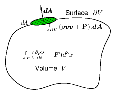
<div class="p"><!----></div>
<a id="tth_fIg7.1">
</a>   <img src="figures/pvolumeint.png" alt="figures/pvolumeint.png" /><a id="pvolumeint">
</a>
  
<div style="text-align:center">Figure 7.1: Integral of momentum flux density across the boundary surface
    <math xmlns="http://www.w3.org/1998/Math/MathML">
<mrow><mo>&part;</mo><mi>V</mi></mrow></math> is equal to minus the integral of  rate of change of
    momentum minus force density over the volume <math xmlns="http://www.w3.org/1998/Math/MathML">
<mrow><mi>V</mi></mrow></math>. The momentum
    flux density includes convective flux and stress tensor parts.<a id="lpvolumeint">
</a></div>

<div class="p"><!----></div>
The conservation of momentum is then
<a id="momnconsv">
</a><br />
<table width="100%"><tr><td align="center">
    <math xmlns="http://www.w3.org/1998/Math/MathML">
    <mstyle displaystyle="true"><mrow>
<mfrac><mrow><mo>&part;</mo></mrow>
<mrow><mo>&part;</mo><mi>t</mi></mrow>
</mfrac>

<msub><mrow><mo>&int;</mo></mrow><mrow><mi>V</mi></mrow>
</msub>
<mi mathvariant="italic">&rho;</mi><mi mathvariant="bold-italic">v</mi>
<msup><mrow><mi>d</mi></mrow><mrow><mn>3</mn></mrow>
</msup>
<mi>x</mi><mo>=</mo>
<msub><mrow><mo>&int;</mo></mrow><mrow><mi>V</mi></mrow>
</msub>
<mi mathvariant="bold-italic">F</mi>
<msup><mrow><mi>d</mi></mrow><mrow><mn>3</mn></mrow>
</msup>
<mi>x</mi><mo>-</mo>
<msub><mrow><mo>&int;</mo></mrow><mrow><mo>&part;</mo><mi>V</mi></mrow>
</msub>
<mo stretchy="false">(</mo><mi mathvariant="italic">&rho;</mi><mi mathvariant="bold-italic">v</mi><mi mathvariant="bold-italic">v</mi><mo>+</mo><mi mathvariant="bold">P</mi><mo stretchy="false">)</mo><mo>.</mo><mi mathvariant="bold-italic">dA</mi><mo>.</mo></mrow>
    </mstyle></math></td><td width="1">
    <math xmlns="http://www.w3.org/1998/Math/MathML">
    <mstyle displaystyle="true"><mrow><mo stretchy="false">(</mo><mn>7</mn><mo>.</mo><mn>2</mn><mo stretchy="false">)</mo></mrow>
    </mstyle></math>
</td></tr></table>


applied to an arbitrary volume and surface, as illustrated in Fig.&nbsp;<a href="chap7.xml#lpvolumeint">7.1</a>.
Just as with mass conservation, we can use Gauss's
divergence<a 
id="Gauss_theorem71413"></a> theorem
to turn the surface integral into a volume integral, and gather the
terms together:
<a id="momnvol">
</a><br />
<table width="100%"><tr><td align="center">
    <math xmlns="http://www.w3.org/1998/Math/MathML">
    <mstyle displaystyle="true"><mrow>
<msub><mrow><mo>&int;</mo></mrow><mrow><mi>V</mi></mrow>
</msub>

<mfrac><mrow><mo>&part;</mo></mrow>
<mrow><mo>&part;</mo><mi>t</mi></mrow>
</mfrac>
<mo stretchy="false">(</mo><mi mathvariant="italic">&rho;</mi><mi mathvariant="bold-italic">v</mi><mo stretchy="false">)</mo><mo>-</mo><mi mathvariant="bold-italic">F</mi><mo>+</mo><mo>&nabla;</mo><mo>.</mo><mo stretchy="false">(</mo><mi mathvariant="italic">&rho;</mi><mi mathvariant="bold-italic">v</mi><mi mathvariant="bold-italic">v</mi><mo>+</mo><mi mathvariant="bold">P</mi><mo stretchy="false">)</mo>
<msup><mrow><mi>d</mi></mrow><mrow><mn>3</mn></mrow>
</msup>
<mi>x</mi><mo>=</mo><mn>0</mn><mo>.</mo></mrow>
    </mstyle></math></td><td width="1">
    <math xmlns="http://www.w3.org/1998/Math/MathML">
    <mstyle displaystyle="true"><mrow><mo stretchy="false">(</mo><mn>7</mn><mo>.</mo><mn>3</mn><mo stretchy="false">)</mo></mrow>
    </mstyle></math>
</td></tr></table>


This equation must hold for any volume <math xmlns="http://www.w3.org/1998/Math/MathML">
<mrow><mi>V</mi></mrow></math>, and the only way for that
to be true is for the integrand to be zero everywhere:
<a id="momngen">
</a><br />
<table width="100%"><tr><td align="center">
    <math xmlns="http://www.w3.org/1998/Math/MathML">
    <mstyle displaystyle="true"><mrow>
<mfrac><mrow><mo>&part;</mo></mrow>
<mrow><mo>&part;</mo><mi>t</mi></mrow>
</mfrac>
<mo stretchy="false">(</mo><mi mathvariant="italic">&rho;</mi><mi mathvariant="bold-italic">v</mi><mo stretchy="false">)</mo><mo>-</mo><mi mathvariant="bold-italic">F</mi><mo>+</mo><mo>&nabla;</mo><mo>.</mo><mo stretchy="false">(</mo><mi mathvariant="italic">&rho;</mi><mi mathvariant="bold-italic">v</mi><mi mathvariant="bold-italic">v</mi><mo>+</mo><mi mathvariant="bold">P</mi><mo stretchy="false">)</mo><mo>=</mo><mn>0</mn><mo>.</mo></mrow>
    </mstyle></math></td><td width="1">
    <math xmlns="http://www.w3.org/1998/Math/MathML">
    <mstyle displaystyle="true"><mrow><mo stretchy="false">(</mo><mn>7</mn><mo>.</mo><mn>4</mn><mo stretchy="false">)</mo></mrow>
    </mstyle></math>
</td></tr></table>


This is the general form of the fluid momentum conservation equation.
If we know what <math xmlns="http://www.w3.org/1998/Math/MathML">
<mrow><mi mathvariant="bold">P</mi></mrow></math> is, then this equation is enough to solve
for <math xmlns="http://www.w3.org/1998/Math/MathML">
<mrow><mi mathvariant="bold-italic">v</mi></mrow></math>. But really we are in the same situation as we were with
the continuity equation. There, we could solve the equation for
<math xmlns="http://www.w3.org/1998/Math/MathML">
<mrow><mi mathvariant="italic">&rho;</mi></mrow></math>, but only if we knew <math xmlns="http://www.w3.org/1998/Math/MathML">
<mrow><mi mathvariant="bold-italic">v</mi></mrow></math>. Now we've got an equation for
<math xmlns="http://www.w3.org/1998/Math/MathML">
<mrow><mi mathvariant="bold-italic">v</mi></mrow></math>, but it depends upon knowing <math xmlns="http://www.w3.org/1998/Math/MathML">
<mrow><mi mathvariant="bold">P</mi></mrow></math>. Intuitively you can
see that this heirarchical process might go on for ever. We can get an
equation for <math xmlns="http://www.w3.org/1998/Math/MathML">
<mrow><mi mathvariant="bold">P</mi></mrow></math> from the conservation of <em>energy</em>, but
that equation will contain a third-order tensor governing the energy
flux<a 
id="energy_flux71414"></a> (conduction etc.). Solving for that requires yet another
equation, and so on. In general, to get a soluble problem we have to
call a halt at some point - a process called
"closure"<a 
id="closure71415"></a>. How and
when we do that decides what sort of fluid equations we end up with.
This closure generally invokes a "constitutive
relation"<a 
id="constitutive_relation71416"></a> between a
property such as stress and the other variables of the fluid such as
density or velocity gradient.

<div class="p"><!----></div>
The kinds of fluids we encounter most in everyday life are
isotropic<a 
id="isotropic71417"></a>. They have no intrinsically preferred
direction.  There are fluids that are anisotropic<a 
id="anisotropic71418"></a>,
for example plasmas or other electrically conducting fluids in
magnetic fields<a 
id="magnetic_field71419"></a>. But for now we set them
aside. Isotropic fluids generally give rise to nearly
symmetric<a 
id="symmetric_stress71420"></a> stress tensors <math xmlns="http://www.w3.org/1998/Math/MathML">
<mrow><mi mathvariant="bold">P</mi></mrow></math>. It is then
helpful to separate out the total stress tensor into a part that is
simply a scalar <math xmlns="http://www.w3.org/1998/Math/MathML">
<mrow><mi>p</mi></mrow></math> times the unit matrix <math xmlns="http://www.w3.org/1998/Math/MathML">
<mrow><mi mathvariant="bold">I</mi></mrow></math> (that's the
isotropic part), and a part <math xmlns="http://www.w3.org/1998/Math/MathML">
<mrow><mi mathvariant="bold-italic">&sigma;</mi></mrow></math> that has zero
<em>trace</em><a 
id="trace__of_matrix71421"></a><a 
id="matrix_trace71422"></a>,
i.e.&nbsp;the sum of its diagonal elements is zero <math xmlns="http://www.w3.org/1998/Math/MathML">
<mrow>
<munder><mo>&sum;</mo><mrow><mi>i</mi></mrow>
</munder>

<msub><mrow><mi mathvariant="italic">&sigma;</mi></mrow><mrow><mi mathvariant="italic">ii</mi></mrow>
</msub>
<mo>=</mo><mn>0</mn></mrow></math>. Thus we write <math xmlns="http://www.w3.org/1998/Math/MathML">
<mrow><mi mathvariant="bold">P</mi><mo>=</mo><mi>p</mi><mi mathvariant="bold">I</mi><mo>+</mo><mi mathvariant="bold-italic">&sigma;</mi></mrow></math>.  Then <math xmlns="http://www.w3.org/1998/Math/MathML">
<mrow><mi>p</mi></mrow></math>
is the <em>pressure</em>.

<div class="p"><!----></div>
<a id="tth_fIg7.2">
</a>   <img src="figures/rateofstrain.png" alt="figures/rateofstrain.png" /><a id="rateofstrain">
</a>
  
<div style="text-align:center">Figure 7.2: The transfer in the <math xmlns="http://www.w3.org/1998/Math/MathML">
<mrow><mi>y</mi></mrow></math>-direction of <math xmlns="http://www.w3.org/1998/Math/MathML">
<mrow><mi>x</mi></mrow></math>-momentum arises
    from the rate of strain <math xmlns="http://www.w3.org/1998/Math/MathML">
<mrow>
<msub><mrow><mi mathvariant="italic">dv</mi></mrow><mrow><mi>x</mi></mrow>
</msub>
<mo stretchy="false">/</mo><mi mathvariant="italic">dy</mi></mrow></math>. The rate of strain tensor is
    the symmetric generalization of this form.<a id="lrateofstrain">
</a></div>

<div class="p"><!----></div>
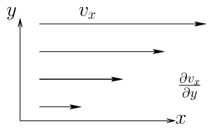
The traceless stress tensor <math xmlns="http://www.w3.org/1998/Math/MathML">
<mrow><mi mathvariant="bold-italic">&sigma;</mi></mrow></math>
for simple fluids arises from viscosity, which relates stress to the
rate of strain tensor<a 
id="rate_of_strain71423"></a>, see Fig.&nbsp;<a href="chap7.xml#lrateofstrain">7.2</a>. The rate of strain tensor
is <math xmlns="http://www.w3.org/1998/Math/MathML">
<mrow>
<mfrac><mrow><mn>1</mn></mrow>
<mrow><mn>2</mn></mrow>
</mfrac>
<mrow><mo>(</mo>
<mfrac><mrow><mo>&part;</mo>
<msub><mrow><mi>v</mi></mrow><mrow><mi>i</mi></mrow>
</msub>
</mrow>
<mrow><mo>&part;</mo>
<msub><mrow><mi>x</mi></mrow><mrow><mi>j</mi></mrow>
</msub>
</mrow>
</mfrac>
<mo>+</mo>
<mfrac><mrow><mo>&part;</mo>
<msub><mrow><mi>v</mi></mrow><mrow><mi>j</mi></mrow>
</msub>
</mrow>
<mrow><mo>&part;</mo>
<msub><mrow><mi>x</mi></mrow><mrow><mi>i</mi></mrow>
</msub>
</mrow>
</mfrac>
<mo>)</mo></mrow></mrow></math>. And <math xmlns="http://www.w3.org/1998/Math/MathML">
<mrow><mi mathvariant="bold-italic">&sigma;</mi></mrow></math> is proportional to
its traceless part
<a id="sigmavisc">
</a><br />
<table width="100%"><tr><td align="center">
    <math xmlns="http://www.w3.org/1998/Math/MathML">
    <mstyle displaystyle="true"><mrow>
<msub><mrow><mi mathvariant="italic">&sigma;</mi></mrow><mrow><mi mathvariant="italic">ij</mi></mrow>
</msub>
<mo>=</mo><mi mathvariant="italic">&mu;</mi><mrow><mo>[</mo><mrow><mo>(</mo>
<mfrac><mrow><mo>&part;</mo>
<msub><mrow><mi>v</mi></mrow><mrow><mi>i</mi></mrow>
</msub>
</mrow>
<mrow><mo>&part;</mo>
<msub><mrow><mi>x</mi></mrow><mrow><mi>j</mi></mrow>
</msub>
</mrow>
</mfrac>
<mo>+</mo>
<mfrac><mrow><mo>&part;</mo>
<msub><mrow><mi>v</mi></mrow><mrow><mi>j</mi></mrow>
</msub>
</mrow>
<mrow><mo>&part;</mo>
<msub><mrow><mi>x</mi></mrow><mrow><mi>i</mi></mrow>
</msub>
</mrow>
</mfrac>
<mo>)</mo></mrow><mo>-</mo>
<mfrac><mrow><mn>2</mn></mrow>
<mrow><mn>3</mn></mrow>
</mfrac>
<mo>&nabla;</mo><mo>.</mo><mi mathvariant="bold-italic">v</mi>
<msub><mrow><mi mathvariant="italic">&delta;</mi></mrow><mrow><mi mathvariant="italic">ij</mi></mrow>
</msub>
<mo>]</mo></mrow><mo>=</mo><mi mathvariant="italic">&mu;</mi>
<msub><mrow><mo>[</mo><mrow><mo>(</mo><mo stretchy="false">(</mo><mo>&nabla;</mo><mi mathvariant="bold-italic">v</mi><mo stretchy="false">)</mo><mo>+</mo><mo stretchy="false">(</mo><mo>&nabla;</mo><mi mathvariant="bold-italic">v</mi>
<msup><mrow><mo stretchy="false">)</mo></mrow><mrow><mi>T</mi></mrow>
</msup>
<mo>)</mo></mrow><mo>-</mo>
<mfrac><mrow><mn>2</mn></mrow>
<mrow><mn>3</mn></mrow>
</mfrac>
<mo stretchy="false">(</mo><mo>&nabla;</mo><mo>.</mo><mi mathvariant="bold-italic">v</mi><mo stretchy="false">)</mo><mi mathvariant="bold">I</mi><mo>]</mo></mrow><mrow><mi mathvariant="italic">ij</mi></mrow>
</msub>
<mo>.</mo></mrow>
    </mstyle></math></td><td width="1">
    <math xmlns="http://www.w3.org/1998/Math/MathML">
    <mstyle displaystyle="true"><mrow><mo stretchy="false">(</mo><mn>7</mn><mo>.</mo><mn>5</mn><mo stretchy="false">)</mo></mrow>
    </mstyle></math>
</td></tr></table>


The constant of proportionality, <math xmlns="http://www.w3.org/1998/Math/MathML">
<mrow><mi mathvariant="italic">&mu;</mi></mrow></math> is the (shear)
<em>viscosity</em><a 
id="viscosity_shear71424"></a>. Here <math xmlns="http://www.w3.org/1998/Math/MathML">
<mrow><mo stretchy="false">(</mo><mo>&nabla;</mo><mi mathvariant="bold-italic">v</mi><mo stretchy="false">)</mo></mrow></math> is a
tensor (dyadic) whose transpose is indicated with a superscript
<math xmlns="http://www.w3.org/1998/Math/MathML">
<mrow><mi>T</mi></mrow></math>. Substituting this expression into the general momentum
conservation equation gives what is called the Navier-Stokes
equation<a 
id="Navier_Stokes71425"></a>.
<a id="NavierStokes">
</a><br />
<table width="100%"><tr><td align="center">
    <math xmlns="http://www.w3.org/1998/Math/MathML">
    <mstyle displaystyle="true"><mrow>
<mfrac><mrow><mo>&part;</mo></mrow>
<mrow><mo>&part;</mo><mi>t</mi></mrow>
</mfrac>
<mo stretchy="false">(</mo><mi mathvariant="italic">&rho;</mi><mi mathvariant="bold-italic">v</mi><mo stretchy="false">)</mo><mo>+</mo><mo>&nabla;</mo><mo>.</mo><mo stretchy="false">(</mo><mi mathvariant="italic">&rho;</mi><mi mathvariant="bold-italic">v</mi><mi mathvariant="bold-italic">v</mi><mo stretchy="false">)</mo><mo>=</mo><mo>-</mo><mo>&nabla;</mo><mo>.</mo><mo stretchy="false">(</mo><mi>p</mi><mi mathvariant="bold">I</mi><mo>+</mo><mi mathvariant="bold-italic">&sigma;</mi><mo stretchy="false">)</mo><mo>+</mo><mi mathvariant="bold-italic">F</mi><mo>=</mo><mo>-</mo><mo>&nabla;</mo><mi>p</mi><mo>-</mo><mi mathvariant="italic">&mu;</mi>
<msup><mrow><mo>&nabla;</mo></mrow><mrow><mn>2</mn></mrow>
</msup>
<mi mathvariant="bold-italic">v</mi><mo>-</mo>
<mfrac><mrow><mn>1</mn></mrow>
<mrow><mn>3</mn></mrow>
</mfrac>
<mi mathvariant="italic">&mu;</mi><mo>&nabla;</mo><mo stretchy="false">(</mo><mo>&nabla;</mo><mo>.</mo><mi mathvariant="bold-italic">v</mi><mo stretchy="false">)</mo><mo>+</mo><mi mathvariant="bold-italic">F</mi><mo>.</mo></mrow>
    </mstyle></math></td><td width="1">
    <math xmlns="http://www.w3.org/1998/Math/MathML">
    <mstyle displaystyle="true"><mrow><mo stretchy="false">(</mo><mn>7</mn><mo>.</mo><mn>6</mn><mo stretchy="false">)</mo></mrow>
    </mstyle></math>
</td></tr></table>


<div class="p"><!----></div>
The closure for the pressure (and viscosity) must generally be
determined by equations of state relating pressure, <math xmlns="http://www.w3.org/1998/Math/MathML">
<mrow><mi>p</mi></mrow></math>, to density, <math xmlns="http://www.w3.org/1998/Math/MathML">
<mrow><mi mathvariant="italic">&rho;</mi></mrow></math>. For example
for an ideal isothermal gas <math xmlns="http://www.w3.org/1998/Math/MathML">
<mrow><mi>p</mi><mo>&prop;</mo><mi mathvariant="italic">&rho;</mi></mrow></math>. Liquids<a 
id="liquid71426"></a>
have an equation of state that amounts approximately to
incompressibility<a 
id="incompressible71427"></a><a 
id="fluid_incompressible71428"></a>,
<math xmlns="http://www.w3.org/1998/Math/MathML">
<mrow><mi mathvariant="italic">&rho;</mi><mo>=</mo><mi mathvariant="italic">const</mi><mo>.</mo></mrow></math>, and they generally have zero volumetric source <math xmlns="http://www.w3.org/1998/Math/MathML">
<mrow><mi>S</mi></mrow></math>. For
such a fluid, the continuity equation shows that the velocity
divergence is zero, <math xmlns="http://www.w3.org/1998/Math/MathML">
<mrow><mo>&nabla;</mo><mo>.</mo><mi mathvariant="bold-italic">v</mi><mo>=</mo><mn>0</mn></mrow></math>. The divergenceless fluid
momentum equation is then simpler.
<a id="Divirgenceless">
</a><br />
<table width="100%"><tr><td align="center">
    <math xmlns="http://www.w3.org/1998/Math/MathML">
    <mstyle displaystyle="true"><mrow>
<mfrac><mrow><mo>&part;</mo></mrow>
<mrow><mo>&part;</mo><mi>t</mi></mrow>
</mfrac>
<mo stretchy="false">(</mo><mi mathvariant="italic">&rho;</mi><mi mathvariant="bold-italic">v</mi><mo stretchy="false">)</mo><mo>+</mo><mo>&nabla;</mo><mo>.</mo><mo stretchy="false">(</mo><mi mathvariant="italic">&rho;</mi><mi mathvariant="bold-italic">v</mi><mi mathvariant="bold-italic">v</mi><mo stretchy="false">)</mo><mo>=</mo><mo>-</mo><mo>&nabla;</mo><mi>p</mi><mo>-</mo><mi mathvariant="italic">&mu;</mi>
<msup><mrow><mo>&nabla;</mo></mrow><mrow><mn>2</mn></mrow>
</msup>
<mi mathvariant="bold-italic">v</mi><mo>+</mo><mi mathvariant="bold-italic">F</mi><mo>.</mo></mrow>
    </mstyle></math></td><td width="1">
    <math xmlns="http://www.w3.org/1998/Math/MathML">
    <mstyle displaystyle="true"><mrow><mo stretchy="false">(</mo><mn>7</mn><mo>.</mo><mn>7</mn><mo stretchy="false">)</mo></mrow>
    </mstyle></math>
</td></tr></table>


And of course if viscosity and body forces are negligible it becomes
even simpler yet. 

<div class="p"><!----></div>
The left hand side of these equations is often
rewritten using the continuity equation with <math xmlns="http://www.w3.org/1998/Math/MathML">
<mrow><mi>S</mi><mo>=</mo><mn>0</mn></mrow></math> to demonstrate
<a id="convectivederiv">
</a><br />
<table width="100%"><tr><td align="center">
    <math xmlns="http://www.w3.org/1998/Math/MathML">
    <mstyle displaystyle="true"><mrow>
<mfrac><mrow><mo>&part;</mo></mrow>
<mrow><mo>&part;</mo><mi>t</mi></mrow>
</mfrac>
<mo stretchy="false">(</mo><mi mathvariant="italic">&rho;</mi><mi mathvariant="bold-italic">v</mi><mo stretchy="false">)</mo><mo>+</mo><mo>&nabla;</mo><mo>.</mo><mo stretchy="false">(</mo><mi mathvariant="italic">&rho;</mi><mi mathvariant="bold-italic">v</mi><mi mathvariant="bold-italic">v</mi><mo stretchy="false">)</mo><mo>=</mo><mi mathvariant="italic">&rho;</mi><mrow><mo>(</mo>
<mfrac><mrow><mo>&part;</mo></mrow>
<mrow><mo>&part;</mo><mi>t</mi></mrow>
</mfrac>
<mi mathvariant="bold-italic">v</mi><mo>+</mo><mi mathvariant="bold-italic">v</mi><mo>.</mo><mo>&nabla;</mo><mi mathvariant="bold-italic">v</mi><mo>)</mo></mrow><mo>.</mo></mrow>
    </mstyle></math></td><td width="1">
    <math xmlns="http://www.w3.org/1998/Math/MathML">
    <mstyle displaystyle="true"><mrow><mo stretchy="false">(</mo><mn>7</mn><mo>.</mo><mn>8</mn><mo stretchy="false">)</mo></mrow>
    </mstyle></math>
</td></tr></table>


Then the second form is recognized as <math xmlns="http://www.w3.org/1998/Math/MathML">
<mrow><mi mathvariant="italic">&rho;</mi></mrow></math> times the convective
derivative <math xmlns="http://www.w3.org/1998/Math/MathML">
<mrow><mo>&part;</mo><mo stretchy="false">/</mo><mo>&part;</mo><mi>t</mi><mo>+</mo><mi mathvariant="bold-italic">v</mi><mo>.</mo><mo>&nabla;</mo></mrow></math> of
<math xmlns="http://www.w3.org/1998/Math/MathML">
<mrow><mi mathvariant="bold-italic">v</mi></mrow></math>. However, the first form is what is called "conservative"
form<a 
id="conservative_form71429"></a>, and it is by far the better form to use
for discrete representation and numerical solution on fixed meshes.

<div class="p"><!----></div>
 <a id="tth_sEc7.2"></a><h2>
7.2&nbsp;&nbsp;Hyperbolic Equations</h2>

<div class="p"><!----></div>
Fluid equations are generally hyperbolic.
Let's start our analysis of such hyperbolic equations<a 
id="hyperbolic72430"></a> by
considering a problem where body force is zero; sources are zero;
viscosity is zero; pressure is related to density by an adiabatic law
<math xmlns="http://www.w3.org/1998/Math/MathML">
<mrow><mi>p</mi>
<msup><mrow><mi mathvariant="italic">&rho;</mi></mrow><mrow><mo>-</mo><mi mathvariant="italic">&gamma;</mi></mrow>
</msup>
<mo>=</mo><mi mathvariant="italic">const</mi><mo>.</mo></mrow></math>; and the configuration is one-dimensional in
space. This is governed then by the following equations.
<a id="onedcompressive">
</a><br />
<table width="100%"><tr><td align="center">
    <math xmlns="http://www.w3.org/1998/Math/MathML">
    <mstyle displaystyle="true"><mrow>
<mtable>
<mtr><mtd columnalign="left"><mrow><mi mathvariant="italic">Continuity</mi><mo>:</mo><mi>&emsp;&emsp;&emsp;&emsp;&emsp;&emsp;</mi></mrow></mtd><mtd columnalign="right"><mrow>
<mfrac><mrow><mo>&part;</mo><mi mathvariant="italic">&rho;</mi></mrow>
<mrow><mo>&part;</mo><mi>t</mi></mrow>
</mfrac>
<mo>+</mo>
<mfrac><mrow><mo>&part;</mo></mrow>
<mrow><mo>&part;</mo><mi>x</mi></mrow>
</mfrac>
<mo stretchy="false">(</mo><mi mathvariant="italic">&rho;</mi><mi>v</mi><mo stretchy="false">)</mo></mrow></mtd><mtd columnalign="center"><mrow><mo>=</mo></mrow></mtd><mtd columnalign="left"><mrow><mn>0</mn></mrow></mtd></mtr>
<mtr><mtd columnalign="left"><mrow><mi mathvariant="italic">Momentum</mi><mo>:</mo><mi>&emsp;&emsp;&emsp;&emsp;&emsp;&emsp;</mi></mrow></mtd><mtd columnalign="right"><mrow>
<mfrac><mrow><mo>&part;</mo></mrow>
<mrow><mo>&part;</mo><mi>t</mi></mrow>
</mfrac>
<mo stretchy="false">(</mo><mi mathvariant="italic">&rho;</mi><mi>v</mi><mo stretchy="false">)</mo><mo>+</mo>
<mfrac><mrow><mo>&part;</mo></mrow>
<mrow><mo>&part;</mo><mi>x</mi></mrow>
</mfrac>
<mo stretchy="false">(</mo><mi mathvariant="italic">&rho;</mi>
<msup><mrow><mi>v</mi></mrow><mrow><mn>2</mn></mrow>
</msup>
<mo stretchy="false">)</mo></mrow></mtd><mtd columnalign="center"><mrow><mo>=</mo></mrow></mtd><mtd columnalign="left"><mrow><mo>-</mo>
<mfrac><mrow><mo>&part;</mo></mrow>
<mrow><mo>&part;</mo><mi>x</mi></mrow>
</mfrac>
<mi>p</mi></mrow></mtd></mtr>
<mtr><mtd columnalign="left"><mrow><mi mathvariant="italic">State</mi><mo>:</mo><mi>&emsp;&emsp;&emsp;&emsp;&emsp;&emsp;</mi></mrow></mtd><mtd columnalign="right"><mrow><mi>p</mi>
<msup><mrow><mi mathvariant="italic">&rho;</mi></mrow><mrow><mo>-</mo><mi mathvariant="italic">&gamma;</mi></mrow>
</msup>
</mrow></mtd><mtd columnalign="center"><mrow><mo>=</mo></mrow></mtd><mtd columnalign="left"><mrow><mi mathvariant="italic">const</mi><mo>.</mo></mrow></mtd></mtr></mtable>

</mrow>
    </mstyle></math></td><td width="1">
    <math xmlns="http://www.w3.org/1998/Math/MathML">
    <mstyle displaystyle="true"><mrow><mo stretchy="false">(</mo><mn>7</mn><mo>.</mo><mn>9</mn><mo stretchy="false">)</mo></mrow>
    </mstyle></math>
</td></tr></table>


These are three equations for three unknowns <math xmlns="http://www.w3.org/1998/Math/MathML">
<mrow><mi mathvariant="italic">&rho;</mi></mrow></math>, <math xmlns="http://www.w3.org/1998/Math/MathML">
<mrow><mi>v</mi></mrow></math>, and
<math xmlns="http://www.w3.org/1998/Math/MathML">
<mrow><mi>p</mi></mrow></math>. They<a 
id="fluid_compressible72431"></a> represent a
compressible<a 
id="compressible_fluid72432"></a> fluid (gas) in a pipe, for
example.  We can eliminate <math xmlns="http://www.w3.org/1998/Math/MathML">
<mrow><mi>p</mi></mrow></math> immediately by writing
<math xmlns="http://www.w3.org/1998/Math/MathML">
<mrow><mi>p</mi><mo>=</mo>
<msub><mrow><mi>p</mi></mrow><mrow><mn>0</mn></mrow>
</msub>

<msup><mrow><mi mathvariant="italic">&rho;</mi></mrow><mrow><mi mathvariant="italic">&gamma;</mi></mrow>
</msup>
<mo stretchy="false">/</mo>
<msubsup><mrow><mi mathvariant="italic">&rho;</mi></mrow><mrow><mn>0</mn> </mrow>
<mrow><mi mathvariant="italic">&gamma;</mi></mrow></msubsup>
</mrow></math>. To retain the conservation
properties, we regard the density, <math xmlns="http://www.w3.org/1998/Math/MathML">
<mrow><mi mathvariant="italic">&rho;</mi></mrow></math>, and <em>momentum
  density</em>, <math xmlns="http://www.w3.org/1998/Math/MathML">
<mrow><mi mathvariant="italic">&rho;</mi><mi>v</mi><mo>=</mo><mi mathvariant="italic">&Gamma;</mi></mrow></math>, as the independent variables, in which
case the equations become
<a id="1dc2">
</a><br />
<table width="100%"><tr><td align="center">
    <math xmlns="http://www.w3.org/1998/Math/MathML">
    <mstyle displaystyle="true"><mrow>
<mtable>
<mtr><mtd columnalign="right"><mrow>
<mfrac><mrow><mo>&part;</mo><mi mathvariant="italic">&rho;</mi></mrow>
<mrow><mo>&part;</mo><mi>t</mi></mrow>
</mfrac>
</mrow></mtd><mtd columnalign="center"><mrow><mo>=</mo></mrow></mtd><mtd columnalign="left"><mrow><mo>-</mo>
<mfrac><mrow><mo>&part;</mo><mi mathvariant="italic">&Gamma;</mi></mrow>
<mrow><mo>&part;</mo><mi>x</mi></mrow>
</mfrac>
</mrow></mtd></mtr>
<mtr><mtd columnalign="right"><mrow>
<mfrac><mrow><mo>&part;</mo><mi mathvariant="italic">&Gamma;</mi></mrow>
<mrow><mo>&part;</mo><mi>t</mi></mrow>
</mfrac>
</mrow></mtd><mtd columnalign="center"><mrow><mo>=</mo></mrow></mtd><mtd columnalign="left"><mrow><mo>-</mo>
<mfrac><mrow><mo>&part;</mo></mrow>
<mrow><mo>&part;</mo><mi>x</mi></mrow>
</mfrac>
<mo stretchy="false">(</mo>
<msup><mrow><mi mathvariant="italic">&Gamma;</mi></mrow><mrow><mn>2</mn></mrow>
</msup>
<mo stretchy="false">/</mo><mi mathvariant="italic">&rho;</mi><mo>+</mo><mo stretchy="false">(</mo>
<msub><mrow><mi>p</mi></mrow><mrow><mn>0</mn></mrow>
</msub>
<mo stretchy="false">/</mo>
<msubsup><mrow><mi mathvariant="italic">&rho;</mi></mrow><mrow><mn>0</mn> </mrow>
<mrow><mi mathvariant="italic">&gamma;</mi></mrow></msubsup>
<mo stretchy="false">)</mo>
<msup><mrow><mi mathvariant="italic">&rho;</mi></mrow><mrow><mi mathvariant="italic">&gamma;</mi></mrow>
</msup>
<mo stretchy="false">)</mo></mrow></mtd></mtr></mtable>

<mo>.</mo></mrow>
    </mstyle></math></td><td width="1">
    <math xmlns="http://www.w3.org/1998/Math/MathML">
    <mstyle displaystyle="true"><mrow><mo stretchy="false">(</mo><mn>7</mn><mo>.</mo><mn>10</mn><mo stretchy="false">)</mo></mrow>
    </mstyle></math>
</td></tr></table>


<div class="p"><!----></div>
We might well want to solve these nonlinear equations
numerically. They are now expressed in a form that is actually the
same for all types of fluid conservation<a 
id="conservation_equation72433"></a> equations:
<a id="hypergeneric">
</a><br />
<table width="100%"><tr><td align="center">
    <math xmlns="http://www.w3.org/1998/Math/MathML">
    <mstyle displaystyle="true"><mrow>
<mfrac><mrow><mo>&part;</mo><mi mathvariant="bold">u</mi></mrow>
<mrow><mo>&part;</mo><mi>t</mi></mrow>
</mfrac>
<mo>=</mo><mo>-</mo>
<mfrac><mrow><mo>&part;</mo><mi mathvariant="bold">f</mi></mrow>
<mrow><mo>&part;</mo><mi>x</mi></mrow>
</mfrac>
<mo>.</mo></mrow>
    </mstyle></math></td><td width="1">
    <math xmlns="http://www.w3.org/1998/Math/MathML">
    <mstyle displaystyle="true"><mrow><mo stretchy="false">(</mo><mn>7</mn><mo>.</mo><mn>11</mn><mo stretchy="false">)</mo></mrow>
    </mstyle></math>
</td></tr></table>


In our particular case
<a id="hypervectors">
</a><br />
<table width="100%"><tr><td align="center">
    <math xmlns="http://www.w3.org/1998/Math/MathML">
    <mstyle displaystyle="true"><mrow><mi mathvariant="bold">u</mi><mo>=</mo><mrow><mo>(</mo>
<mtable>
<mtr><mtd columnalign="center"><mrow><mi mathvariant="italic">&rho;</mi></mrow></mtd></mtr>
<mtr><mtd columnalign="center"><mrow><mi mathvariant="italic">&Gamma;</mi></mrow></mtd></mtr></mtable>

<mo>)</mo></mrow><mo>,</mo><mi>&emsp;&emsp;&emsp;&emsp;&emsp;&emsp;</mi>
<mtext>and</mtext>
<mi>&emsp;&emsp;&emsp;</mi><mi mathvariant="bold">f</mi><mo>=</mo><mrow><mo>(</mo>
<mtable>
<mtr><mtd columnalign="center"><mrow><mi mathvariant="italic">&Gamma;</mi></mrow></mtd></mtr>
<mtr><mtd columnalign="center"><mrow>
<msup><mrow><mi mathvariant="italic">&Gamma;</mi></mrow><mrow><mn>2</mn></mrow>
</msup>
<mo stretchy="false">/</mo><mi mathvariant="italic">&rho;</mi><mo>+</mo><mo stretchy="false">(</mo>
<msub><mrow><mi>p</mi></mrow><mrow><mn>0</mn></mrow>
</msub>
<mo stretchy="false">/</mo>
<msubsup><mrow><mi mathvariant="italic">&rho;</mi></mrow><mrow><mn>0</mn> </mrow>
<mrow><mi mathvariant="italic">&gamma;</mi></mrow></msubsup>
<mo stretchy="false">)</mo>
<msup><mrow><mi mathvariant="italic">&rho;</mi></mrow><mrow><mi mathvariant="italic">&gamma;</mi></mrow>
</msup>
</mrow></mtd></mtr></mtable>

<mo>)</mo></mrow></mrow>
    </mstyle></math></td><td width="1">
    <math xmlns="http://www.w3.org/1998/Math/MathML">
    <mstyle displaystyle="true"><mrow><mo stretchy="false">(</mo><mn>7</mn><mo>.</mo><mn>12</mn><mo stretchy="false">)</mo></mrow>
    </mstyle></math>
</td></tr></table>


are the state vector<a 
id="state_vector72434"></a> and the flux
vector<a 
id="flux_vector72435"></a> respectively. Since the flux vector is a
function of the state vector, we can use the chain rule to write the
equations as
<a id="hypermatrix">
</a><br />
<table width="100%"><tr><td align="center">
    <math xmlns="http://www.w3.org/1998/Math/MathML">
    <mstyle displaystyle="true"><mrow>
<mfrac><mrow><mo>&part;</mo><mi mathvariant="bold">u</mi></mrow>
<mrow><mo>&part;</mo><mi>t</mi></mrow>
</mfrac>
<mo>=</mo><mo>-</mo>
<mfrac><mrow><mo>&part;</mo><mi mathvariant="bold">f</mi></mrow>
<mrow><mo>&part;</mo><mi mathvariant="bold">u</mi></mrow>
</mfrac>

<mfrac><mrow><mo>&part;</mo><mi mathvariant="bold">u</mi></mrow>
<mrow><mo>&part;</mo><mi>x</mi></mrow>
</mfrac>
<mo>=</mo><mo>-</mo>
<munder><mo>&sum;</mo><mrow><mi>m</mi><mo>=</mo><mn>1</mn><mo>,</mo><mi>M</mi></mrow>
</munder>

<mfrac><mrow><mo>&part;</mo><mi mathvariant="bold">f</mi></mrow>
<mrow><mo>&part;</mo>
<msub><mrow><mi>u</mi></mrow><mrow><mi>m</mi></mrow>
</msub>
</mrow>
</mfrac>

<mfrac><mrow><mo>&part;</mo>
<msub><mrow><mi>u</mi></mrow><mrow><mi>m</mi></mrow>
</msub>
</mrow>
<mrow><mo>&part;</mo><mi>x</mi></mrow>
</mfrac>
<mo>=</mo><mo>-</mo><mi mathvariant="bold">J</mi>
<mfrac><mrow><mo>&part;</mo><mi mathvariant="bold">u</mi></mrow>
<mrow><mo>&part;</mo><mi>x</mi></mrow>
</mfrac>
<mo>.</mo></mrow>
    </mstyle></math></td><td width="1">
    <math xmlns="http://www.w3.org/1998/Math/MathML">
    <mstyle displaystyle="true"><mrow><mo stretchy="false">(</mo><mn>7</mn><mo>.</mo><mn>13</mn><mo stretchy="false">)</mo></mrow>
    </mstyle></math>
</td></tr></table>


Here, the Jacobian<a 
id="Jacobian_matrix72436"></a><a 
id="matrix_Jacobian72437"></a> matrix
<math xmlns="http://www.w3.org/1998/Math/MathML">
<mrow><mi mathvariant="bold">J</mi><mo>=</mo><mo>&part;</mo><mi mathvariant="bold">f</mi><mo stretchy="false">/</mo><mo>&part;</mo><mi mathvariant="bold">u</mi></mrow></math> has size <math xmlns="http://www.w3.org/1998/Math/MathML">
<mrow><mi>M</mi><mo>&times;</mo><mi>M</mi><mo>=</mo><mn>2</mn><mo>&times;</mo><mn>2</mn></mrow></math> and is explicitly
<a id="hyperjac">
</a><br />
<table width="100%"><tr><td align="center">
    <math xmlns="http://www.w3.org/1998/Math/MathML">
    <mstyle displaystyle="true"><mrow><mi mathvariant="bold">J</mi><mo>=</mo><mrow><mo>(</mo>
<mtable>
<mtr><mtd columnalign="center"><mrow><mn>0</mn></mrow></mtd><mtd columnalign="center"><mrow><mn>1</mn></mrow></mtd></mtr>
<mtr><mtd columnalign="center"><mrow><mo>-</mo>
<msup><mrow><mi mathvariant="italic">&Gamma;</mi></mrow><mrow><mn>2</mn></mrow>
</msup>
<mo stretchy="false">/</mo>
<msup><mrow><mi mathvariant="italic">&rho;</mi></mrow><mrow><mn>2</mn></mrow>
</msup>
<mo>+</mo><mi mathvariant="italic">&gamma;</mi><mo stretchy="false">(</mo>
<msub><mrow><mi>p</mi></mrow><mrow><mn>0</mn></mrow>
</msub>
<mo stretchy="false">/</mo>
<msubsup><mrow><mi mathvariant="italic">&rho;</mi></mrow><mrow><mn>0</mn> </mrow>
<mrow><mi mathvariant="italic">&gamma;</mi></mrow></msubsup>
<mo stretchy="false">)</mo>
<msup><mrow><mi mathvariant="italic">&rho;</mi></mrow><mrow><mi mathvariant="italic">&gamma;</mi><mo>-</mo><mn>1</mn></mrow>
</msup>
</mrow></mtd><mtd columnalign="center"><mrow><mn>2</mn><mi mathvariant="italic">&Gamma;</mi><mo stretchy="false">/</mo><mi mathvariant="italic">&rho;</mi></mrow></mtd></mtr></mtable>

<mo>)</mo></mrow><mo>.</mo></mrow>
    </mstyle></math></td><td width="1">
    <math xmlns="http://www.w3.org/1998/Math/MathML">
    <mstyle displaystyle="true"><mrow><mo stretchy="false">(</mo><mn>7</mn><mo>.</mo><mn>14</mn><mo stretchy="false">)</mo></mrow>
    </mstyle></math>
</td></tr></table>


The Jacobian matrix quite generally embodies the differential equation
by relating time-derivates to space-derivatives of the state vector,
through eq.&nbsp;(<a href="chap7.xml#hypermatrix">7.13</a>): <math xmlns="http://www.w3.org/1998/Math/MathML">
<mrow>
<mfrac><mrow><mo>&part;</mo><mi mathvariant="bold">u</mi></mrow>
<mrow><mo>&part;</mo><mi>t</mi></mrow>
</mfrac>
<mo>=</mo><mo>-</mo><mi mathvariant="bold">J</mi>
<mfrac><mrow><mo>&part;</mo><mi mathvariant="bold">u</mi></mrow>
<mrow><mo>&part;</mo><mi>x</mi></mrow>
</mfrac>
</mrow></math>.

<div class="p"><!----></div>
Writing for convenience
<math xmlns="http://www.w3.org/1998/Math/MathML">
<mrow><mi mathvariant="italic">&Gamma;</mi><mo stretchy="false">/</mo><mi mathvariant="italic">&rho;</mi><mo>=</mo><mi>v</mi></mrow></math>, and <math xmlns="http://www.w3.org/1998/Math/MathML">
<mrow><mi mathvariant="italic">&gamma;</mi><mo stretchy="false">(</mo>
<msub><mrow><mi>p</mi></mrow><mrow><mn>0</mn></mrow>
</msub>
<mo stretchy="false">/</mo>
<msubsup><mrow><mi mathvariant="italic">&rho;</mi></mrow><mrow><mn>0</mn> </mrow>
<mrow><mi mathvariant="italic">&gamma;</mi></mrow></msubsup>
<mo stretchy="false">)</mo>
<msup><mrow><mi mathvariant="italic">&rho;</mi></mrow><mrow><mi mathvariant="italic">&gamma;</mi><mo>-</mo><mn>1</mn></mrow>
</msup>
<mo>=</mo>
<msubsup><mrow><mi>c</mi></mrow><mrow><mi>s</mi> </mrow>
<mrow><mn>2</mn></mrow></msubsup>
</mrow></math>,
the eigenvalues<a 
id="eigenvalue_of_Jacobian72438"></a> of <math xmlns="http://www.w3.org/1998/Math/MathML">
<mrow><mi mathvariant="bold">J</mi></mrow></math> are then solutions of
<a id="Jeigen">
</a><br />
<table width="100%"><tr><td align="center">
    <math xmlns="http://www.w3.org/1998/Math/MathML">
    <mstyle displaystyle="true"><mrow><mrow><mo>|</mo>
<mtable>
<mtr><mtd columnalign="center"><mrow><mo>-</mo><mi mathvariant="italic">&lambda;</mi></mrow></mtd><mtd columnalign="center"><mrow><mn>1</mn></mrow></mtd></mtr>
<mtr><mtd columnalign="center"><mrow><mo>-</mo>
<msup><mrow><mi>v</mi></mrow><mrow><mn>2</mn></mrow>
</msup>
<mo>+</mo>
<msubsup><mrow><mi>c</mi></mrow><mrow><mi>s</mi> </mrow>
<mrow><mn>2</mn></mrow></msubsup>
</mrow></mtd><mtd columnalign="center"><mrow><mo>-</mo><mi mathvariant="italic">&lambda;</mi><mo>+</mo><mn>2</mn><mi>v</mi></mrow></mtd></mtr></mtable>

<mo>|</mo></mrow><mo>=</mo>
<msup><mrow><mi mathvariant="italic">&lambda;</mi></mrow><mrow><mn>2</mn></mrow>
</msup>
<mo>-</mo><mn>2</mn><mi>v</mi><mi mathvariant="italic">&lambda;</mi><mo>+</mo>
<msup><mrow><mi>v</mi></mrow><mrow><mn>2</mn></mrow>
</msup>
<mo>-</mo>
<msubsup><mrow><mi>c</mi></mrow><mrow><mi>s</mi> </mrow>
<mrow><mn>2</mn></mrow></msubsup>
<mo>=</mo><mn>0</mn><mo>,</mo></mrow>
    </mstyle></math></td><td width="1">
    <math xmlns="http://www.w3.org/1998/Math/MathML">
    <mstyle displaystyle="true"><mrow><mo stretchy="false">(</mo><mn>7</mn><mo>.</mo><mn>15</mn><mo stretchy="false">)</mo></mrow>
    </mstyle></math>
</td></tr></table>


which are
<a id="Jeigensol">
</a><br />
<table width="100%"><tr><td align="center">
    <math xmlns="http://www.w3.org/1998/Math/MathML">
    <mstyle displaystyle="true"><mrow><mi mathvariant="italic">&lambda;</mi><mo>=</mo><mi>v</mi><mo>&PlusMinus;</mo>
<msub><mrow><mi>c</mi></mrow><mrow><mi>s</mi></mrow>
</msub>
<mo>.</mo></mrow>
    </mstyle></math></td><td width="1">
    <math xmlns="http://www.w3.org/1998/Math/MathML">
    <mstyle displaystyle="true"><mrow><mo stretchy="false">(</mo><mn>7</mn><mo>.</mo><mn>16</mn><mo stretchy="false">)</mo></mrow>
    </mstyle></math>
</td></tr></table>


For small density perturbations, <math xmlns="http://www.w3.org/1998/Math/MathML">
<mrow>
<msubsup><mrow><mi>c</mi></mrow><mrow><mi>s</mi> </mrow>
<mrow><mn>2</mn></mrow></msubsup>
<mo>=</mo><mi mathvariant="italic">&gamma;</mi><mo stretchy="false">(</mo>
<msub><mrow><mi>p</mi></mrow><mrow><mn>0</mn></mrow>
</msub>
<mo stretchy="false">/</mo>
<msubsup><mrow><mi mathvariant="italic">&rho;</mi></mrow><mrow><mn>0</mn> </mrow>
<mrow><mi mathvariant="italic">&gamma;</mi></mrow></msubsup>
<mo stretchy="false">)</mo>
<msup><mrow><mi mathvariant="italic">&rho;</mi></mrow><mrow><mi mathvariant="italic">&gamma;</mi><mo>-</mo><mn>1</mn></mrow>
</msup>
<mo>&ap;</mo><mi mathvariant="italic">&gamma;</mi>
<msub><mrow><mi>p</mi></mrow><mrow><mn>0</mn></mrow>
</msub>
<mo stretchy="false">/</mo>
<msub><mrow><mi mathvariant="italic">&rho;</mi></mrow><mrow><mn>0</mn></mrow>
</msub>
</mrow></math>, which
gives the usual definition of the (small-amplitude) sound speed
<math xmlns="http://www.w3.org/1998/Math/MathML">
<mrow>
<msub><mrow><mi>c</mi></mrow><mrow><mi>s</mi></mrow>
</msub>
<mo>=</mo><msqrt><mrow><mi mathvariant="italic">&gamma;</mi>
<msub><mrow><mi>p</mi></mrow><mrow><mn>0</mn></mrow>
</msub>
<mo stretchy="false">/</mo>
<msub><mrow><mi mathvariant="italic">&rho;</mi></mrow><mrow><mn>0</mn></mrow>
</msub>
</mrow></msqrt></mrow></math>. 

<div class="p"><!----></div>
The fact that the eigenvalues are real<a 
id="eigenvalue_real72439"></a> is a
demonstration that the system of equations is
<em>hyperbolic</em><a 
id="hyperbolic_Jacobian_eigenvalue72440"></a>. The
eigenvalues indicate the speed<a 
id="wave_propagation72441"></a> of
propagation of disturbances. In this fluid they propagate at the speed
of sound<a 
id="speed_of_sound72442"></a> measured in the rest-frame of the fluid.

<div class="p"><!----></div>
 <a id="tth_sEc7.3"></a><h2>
7.3&nbsp;&nbsp;Finite Differences and Stability</h2>

<div class="p"><!----></div>
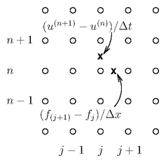
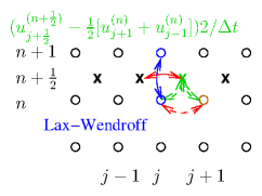
Now let's consider possible finite difference representations of the
equations<a 
id="hyperbolic_finite_difference73443"></a>. We notice that the
simplest time differences give the time derivative
<math xmlns="http://www.w3.org/1998/Math/MathML">
<mrow><mo stretchy="false">(</mo>
<msubsup><mrow><mi mathvariant="bold">u</mi></mrow><mrow><mi>j</mi> </mrow>
<mrow><mo stretchy="false">(</mo><mi>n</mi><mo>+</mo><mn>1</mn><mo stretchy="false">)</mo></mrow></msubsup>
<mo>-</mo>
<msubsup><mrow><mi mathvariant="bold">u</mi></mrow><mrow><mi>j</mi> </mrow>
<mrow><mo stretchy="false">(</mo><mi>n</mi><mo stretchy="false">)</mo></mrow></msubsup>
<mo stretchy="false">)</mo><mo stretchy="false">/</mo><mi mathvariant="italic">&Delta;</mi><mi>t</mi></mrow></math> effectively at time
<math xmlns="http://www.w3.org/1998/Math/MathML">
<mrow><mi>n</mi><mo>+</mo><mn>1</mn><mo stretchy="false">/</mo><mn>2</mn></mrow></math> but position <math xmlns="http://www.w3.org/1998/Math/MathML">
<mrow><mi>j</mi></mrow></math>, and the simplest space difference gives a derivative
<math xmlns="http://www.w3.org/1998/Math/MathML">
<mrow><mo stretchy="false">(</mo>
<msubsup><mrow><mi mathvariant="bold">f</mi></mrow><mrow><mi>j</mi><mo>+</mo><mn>1</mn> </mrow>
<mrow><mo stretchy="false">(</mo><mi>n</mi><mo stretchy="false">)</mo></mrow></msubsup>
<mo>-</mo>
<msubsup><mrow><mi mathvariant="bold">f</mi></mrow><mrow><mi>j</mi> </mrow>
<mrow><mo stretchy="false">(</mo><mi>n</mi><mo stretchy="false">)</mo></mrow></msubsup>
<mo stretchy="false">)</mo><mo stretchy="false">/</mo><mi mathvariant="italic">&Delta;</mi><mi>x</mi></mrow></math> at position
<math xmlns="http://www.w3.org/1998/Math/MathML">
<mrow><mi>j</mi><mo>+</mo><mn>1</mn><mo stretchy="false">/</mo><mn>2</mn></mrow></math>. These expressions don't line up with one another so if we use
them, we'll certainly have only first order accuracy. See Fig.&nbsp;<a href="chap7.xml#fluidmeshl">7.3</a>. 

<div class="p"><!----></div>
<a id="tth_fIg7.3">
</a>    <img src="figures/fluidmesh.png" alt="figures/fluidmesh.png" /><a id="fluidmesh">
</a>
  
<div style="text-align:center">Figure 7.3: Derivatives in time (<math xmlns="http://www.w3.org/1998/Math/MathML">
<mrow><mi>n</mi></mrow></math>) and space (<math xmlns="http://www.w3.org/1998/Math/MathML">
<mrow><mi>j</mi></mrow></math>) implemented as
    finite differences give rise to values at the half-mesh points
    <b>x</b>.<a id="fluidmeshl">
</a></div>

<div class="p"><!----></div>
We could try to
fix that by taking centered derivatives; but it turns out that may
make things worse. The scheme may become unstable. But how do we
analyse stability for this fluid? We have multiple
coupled<a 
id="coupled_equations73444"></a> dependent
variables. How do we deal with that?
The answer, in summary, is that we find the combinations of dependent
variables that behave in a way that is approximately uncoupled from
the other combinations of dependent variables - in other words, the
characteristic <em>modes</em> of the system. Then we analyse the Von
Neumann stability<a 
id="Von_Neumann_stability73445"></a> of those modes separately.

<div class="p"><!----></div>
If the Jacobian matrix is independent of position, then it is possible
to change the dependent variables to new combinations of variables,
each of which is <em>uncoupled</em><a 
id="uncoupled_representation73446"></a> from the other
combinations<a href="footnote.xml#tthFtNtAEC" id="tthFrefAEC"><math xmlns="http://www.w3.org/1998/Math/MathML">
<mrow>
<msup><mrow></mrow><mrow><mn>42</mn></mrow>
</msup>
</mrow></math></a>. The new combination to use consists of the
<em>eigenvectors</em> of the matrix <math xmlns="http://www.w3.org/1998/Math/MathML">
<mrow><mi mathvariant="bold">J</mi></mrow></math>.

<div class="p"><!----></div>
Let's illustrate this with our fluid. Consider the
eigenvalues<a 
id="eigenvalue73447"></a> <math xmlns="http://www.w3.org/1998/Math/MathML">
<mrow><mi mathvariant="italic">&lambda;</mi><mo>=</mo><mi>v</mi><mo>&PlusMinus;</mo>
<msub><mrow><mi>c</mi></mrow><mrow><mi>s</mi></mrow>
</msub>
</mrow></math>. For each eigenvalue,
the eigenvector<a 
id="eigenvector73448"></a>, which is the solution of the
homogeneous equation <math xmlns="http://www.w3.org/1998/Math/MathML">
<mrow><mo stretchy="false">(</mo><mi mathvariant="bold">J</mi><mo>-</mo><mi mathvariant="italic">&lambda;</mi><mi mathvariant="bold">I</mi><mo stretchy="false">)</mo><mi mathvariant="bold">e</mi><mo>=</mo><mn>0</mn></mrow></math>, must give
zero when multiplied by any of the rows of the combined matrix
<math xmlns="http://www.w3.org/1998/Math/MathML">
<mrow><mo stretchy="false">(</mo><mi mathvariant="bold">J</mi><mo>-</mo><mi mathvariant="italic">&lambda;</mi><mi mathvariant="bold">I</mi><mo stretchy="false">)</mo></mrow></math>. Using the top row, which becomes <math xmlns="http://www.w3.org/1998/Math/MathML">
<mrow><mo stretchy="false">(</mo><mo>-</mo><mo stretchy="false">[</mo><mi>v</mi><mo>&PlusMinus;</mo>
<msub><mrow><mi>c</mi></mrow><mrow><mi>s</mi></mrow>
</msub>
<mo stretchy="false">]</mo><mo>,</mo><mn>1</mn><mo stretchy="false">)</mo></mrow></math> we find that the eigenvector is proportional to
<a id="Jeigenvec">
</a><br />
<table width="100%"><tr><td align="center">
    <math xmlns="http://www.w3.org/1998/Math/MathML">
    <mstyle displaystyle="true"><mrow>
<msub><mrow><mi mathvariant="bold">e</mi></mrow><mrow><mo>&PlusMinus;</mo></mrow>
</msub>
<mo>=</mo><mrow><mo>(</mo>
<mtable>
<mtr><mtd columnalign="center"><mrow><mn>1</mn></mrow></mtd></mtr>
<mtr><mtd columnalign="center"><mrow><mi>v</mi><mo>&PlusMinus;</mo>
<msub><mrow><mi>c</mi></mrow><mrow><mi>s</mi></mrow>
</msub>
</mrow></mtd></mtr></mtable>

<mo>)</mo></mrow></mrow>
    </mstyle></math></td><td width="1">
    <math xmlns="http://www.w3.org/1998/Math/MathML">
    <mstyle displaystyle="true"><mrow><mo stretchy="false">(</mo><mn>7</mn><mo>.</mo><mn>17</mn><mo stretchy="false">)</mo></mrow>
    </mstyle></math>
</td></tr></table>


Now we can express any vector state as the sum of two coefficients
<math xmlns="http://www.w3.org/1998/Math/MathML">
<mrow>
<msub><mrow><mi>q</mi></mrow><mrow><mo>&PlusMinus;</mo></mrow>
</msub>
</mrow></math> times the two eigenvectors<a href="footnote.xml#tthFtNtAED" id="tthFrefAED"><math xmlns="http://www.w3.org/1998/Math/MathML">
<mrow>
<msup><mrow></mrow><mrow><mn>43</mn></mrow>
</msup>
</mrow></math></a>
<math xmlns="http://www.w3.org/1998/Math/MathML">
<mrow><mi mathvariant="bold">u</mi><mo>=</mo>
<msub><mrow><mi>q</mi></mrow><mrow><mo>+</mo></mrow>
</msub>

<msub><mrow><mi mathvariant="bold">e</mi></mrow><mrow><mo>+</mo></mrow>
</msub>
<mo>+</mo>
<msub><mrow><mi>q</mi></mrow><mrow><mo>-</mo></mrow>
</msub>

<msub><mrow><mi mathvariant="bold">e</mi></mrow><mrow><mo>-</mo></mrow>
</msub>
</mrow></math> or written out
<a id="eigendecomp">
</a><br />
<table width="100%"><tr><td align="center">
    <math xmlns="http://www.w3.org/1998/Math/MathML">
    <mstyle displaystyle="true"><mrow><mrow><mo>(</mo>
<mtable>
<mtr><mtd columnalign="center"><mrow><mi mathvariant="italic">&rho;</mi></mrow></mtd></mtr>
<mtr><mtd columnalign="center"><mrow><mi mathvariant="italic">&Gamma;</mi></mrow></mtd></mtr></mtable>

<mo>)</mo></mrow><mo>=</mo>
<msub><mrow><mi>q</mi></mrow><mrow><mo>+</mo></mrow>
</msub>
<mrow><mo>(</mo>
<mtable>
<mtr><mtd columnalign="center"><mrow><mn>1</mn></mrow></mtd></mtr>
<mtr><mtd columnalign="center"><mrow><mi>v</mi><mo>+</mo>
<msub><mrow><mi>c</mi></mrow><mrow><mi>s</mi></mrow>
</msub>
</mrow></mtd></mtr></mtable>

<mo>)</mo></mrow><mo>+</mo>
<msub><mrow><mi>q</mi></mrow><mrow><mo>-</mo></mrow>
</msub>
<mrow><mo>(</mo>
<mtable>
<mtr><mtd columnalign="center"><mrow><mn>1</mn></mrow></mtd></mtr>
<mtr><mtd columnalign="center"><mrow><mi>v</mi><mo>-</mo>
<msub><mrow><mi>c</mi></mrow><mrow><mi>s</mi></mrow>
</msub>
</mrow></mtd></mtr></mtable>

<mo>)</mo></mrow><mo>.</mo></mrow>
    </mstyle></math></td><td width="1">
    <math xmlns="http://www.w3.org/1998/Math/MathML">
    <mstyle displaystyle="true"><mrow><mo stretchy="false">(</mo><mn>7</mn><mo>.</mo><mn>18</mn><mo stretchy="false">)</mo></mrow>
    </mstyle></math>
</td></tr></table>


[The coefficient values are <math xmlns="http://www.w3.org/1998/Math/MathML">
<mrow>
<msub><mrow><mi>q</mi></mrow><mrow><mo>&PlusMinus;</mo></mrow>
</msub>
<mo>=</mo><mo stretchy="false">[</mo><mi mathvariant="italic">&rho;</mi><mo stretchy="false">(</mo><mi>v</mi><mo>&mp;</mo>
<msub><mrow><mi>c</mi></mrow><mrow><mi>s</mi></mrow>
</msub>
<mo stretchy="false">)</mo><mo>-</mo><mi mathvariant="italic">&Gamma;</mi><mo stretchy="false">]</mo><mo stretchy="false">/</mo><mo stretchy="false">(</mo><mo>&PlusMinus;</mo><mn>2</mn>
<msub><mrow><mi>c</mi></mrow><mrow><mi>s</mi></mrow>
</msub>
<mo stretchy="false">)</mo></mrow></math> but we don't need to know that.] The quantities <math xmlns="http://www.w3.org/1998/Math/MathML">
<mrow>
<msub><mrow><mi>q</mi></mrow><mrow><mo>&PlusMinus;</mo></mrow>
</msub>
</mrow></math>
can be considered to be the coefficients of the new
vector representation <math xmlns="http://www.w3.org/1998/Math/MathML">
<mrow><mi mathvariant="bold">q</mi><mo>=</mo><mrow><mo>(</mo>
<mfrac linethickness="0"><mrow>
<msub><mrow><mi>q</mi></mrow><mrow><mo>+</mo></mrow>
</msub>
</mrow>
<mrow>
<msub><mrow><mi>q</mi></mrow><mrow><mo>-</mo></mrow>
</msub>
</mrow>
</mfrac>
<mo>)</mo></mrow></mrow></math>, by which
the state can be expressed.
Then the result of multiplying <math xmlns="http://www.w3.org/1998/Math/MathML">
<mrow><mi mathvariant="bold">u</mi></mrow></math> by the Jacobian matrix<a 
id="matrix_Jacobian73449"></a> can be
written in terms of the new set of <math xmlns="http://www.w3.org/1998/Math/MathML">
<mrow><mi>q</mi></mrow></math>-coefficients as follows,
<a id="Jtimeseig">
</a><br />
<table width="100%"><tr><td align="center">
    <math xmlns="http://www.w3.org/1998/Math/MathML">
    <mstyle displaystyle="true"><mrow><mi mathvariant="bold">J</mi><mi mathvariant="bold">u</mi><mo>=</mo>
<msub><mrow><mi>q</mi></mrow><mrow><mo>+</mo></mrow>
</msub>
<mi mathvariant="bold">J</mi>
<msub><mrow><mi mathvariant="bold">e</mi></mrow><mrow><mo>+</mo></mrow>
</msub>
<mo>+</mo>
<msub><mrow><mi>q</mi></mrow><mrow><mo>-</mo></mrow>
</msub>
<mi mathvariant="bold">J</mi>
<msub><mrow><mi mathvariant="bold">e</mi></mrow><mrow><mo>-</mo></mrow>
</msub>
<mo>=</mo>
<msub><mrow><mi>q</mi></mrow><mrow><mo>+</mo></mrow>
</msub>

<msub><mrow><mi mathvariant="italic">&lambda;</mi></mrow><mrow><mo>+</mo></mrow>
</msub>

<msub><mrow><mi mathvariant="bold">e</mi></mrow><mrow><mo>+</mo></mrow>
</msub>
<mo>+</mo>
<msub><mrow><mi>q</mi></mrow><mrow><mo>-</mo></mrow>
</msub>

<msub><mrow><mi mathvariant="italic">&lambda;</mi></mrow><mrow><mo>-</mo></mrow>
</msub>

<msub><mrow><mi mathvariant="bold">e</mi></mrow><mrow><mo>-</mo></mrow>
</msub>
<mi>&ensp;&ensp;</mi><mo>.</mo></mrow>
    </mstyle></math></td><td width="1">
    <math xmlns="http://www.w3.org/1998/Math/MathML">
    <mstyle displaystyle="true"><mrow><mo stretchy="false">(</mo><mn>7</mn><mo>.</mo><mn>19</mn><mo stretchy="false">)</mo></mrow>
    </mstyle></math>
</td></tr></table>


This shows that the vector of eigenvalue coefficients giving
<math xmlns="http://www.w3.org/1998/Math/MathML">
<mrow><mi mathvariant="bold">J</mi><mi mathvariant="bold">u</mi></mrow></math> is <math xmlns="http://www.w3.org/1998/Math/MathML">
<mrow><mrow><mo>(</mo>
<mfrac linethickness="0"><mrow>
<msub><mrow><mi>q</mi></mrow><mrow><mo>+</mo></mrow>
</msub>

<msub><mrow><mi mathvariant="italic">&lambda;</mi></mrow><mrow><mo>+</mo></mrow>
</msub>
</mrow>
<mrow>
<msub><mrow><mi>q</mi></mrow><mrow><mo>-</mo></mrow>
</msub>

<msub><mrow><mi mathvariant="italic">&lambda;</mi></mrow><mrow><mo>-</mo></mrow>
</msub>
</mrow>
</mfrac>
<mo>)</mo></mrow></mrow></math>.  So
in terms of the new <math xmlns="http://www.w3.org/1998/Math/MathML">
<mrow><mi>q</mi></mrow></math>-representation
<a id="NewJ">
</a><br />
<table width="100%"><tr><td align="center">
    <math xmlns="http://www.w3.org/1998/Math/MathML">
    <mstyle displaystyle="true"><mrow>
<mover><mrow><mi mathvariant="bold">J</mi></mrow>
<mo>&OverBar;</mo></mover>
<mi mathvariant="bold">q</mi><mo>=</mo><mrow><mo>(</mo>
<mfrac linethickness="0"><mrow>
<msub><mrow><mi>q</mi></mrow><mrow><mo>+</mo></mrow>
</msub>

<msub><mrow><mi mathvariant="italic">&lambda;</mi></mrow><mrow><mo>+</mo></mrow>
</msub>
</mrow>
<mrow>
<msub><mrow><mi>q</mi></mrow><mrow><mo>-</mo></mrow>
</msub>

<msub><mrow><mi mathvariant="italic">&lambda;</mi></mrow><mrow><mo>-</mo></mrow>
</msub>
</mrow>
</mfrac>
<mo>)</mo></mrow><mo>=</mo><mrow><mo>(</mo>
<mtable>
<mtr><mtd columnalign="center"><mrow>
<msub><mrow><mi mathvariant="italic">&lambda;</mi></mrow><mrow><mo>+</mo></mrow>
</msub>
</mrow></mtd><mtd columnalign="center"><mrow><mn>0</mn></mrow></mtd></mtr>
<mtr><mtd columnalign="center"><mrow><mn>0</mn></mrow></mtd><mtd columnalign="center"><mrow>
<msub><mrow><mi mathvariant="italic">&lambda;</mi></mrow><mrow><mo>-</mo></mrow>
</msub>
</mrow></mtd></mtr></mtable>

<mo>)</mo></mrow><mrow><mo>(</mo>
<mtable>
<mtr><mtd columnalign="center"><mrow>
<msub><mrow><mi>q</mi></mrow><mrow><mo>+</mo></mrow>
</msub>
</mrow></mtd></mtr>
<mtr><mtd columnalign="center"><mrow>
<msub><mrow><mi>q</mi></mrow><mrow><mo>-</mo></mrow>
</msub>
</mrow></mtd></mtr></mtable>

<mo>)</mo></mrow><mo>.</mo></mrow>
    </mstyle></math></td><td width="1">
    <math xmlns="http://www.w3.org/1998/Math/MathML">
    <mstyle displaystyle="true"><mrow><mo stretchy="false">(</mo><mn>7</mn><mo>.</mo><mn>20</mn><mo stretchy="false">)</mo></mrow>
    </mstyle></math>
</td></tr></table>


In this <math xmlns="http://www.w3.org/1998/Math/MathML">
<mrow><mi>q</mi></mrow></math>-representation, the operator <math xmlns="http://www.w3.org/1998/Math/MathML">
<mrow><mi mathvariant="bold">J</mi></mrow></math>, is represented by
a different matrix <math xmlns="http://www.w3.org/1998/Math/MathML">
<mrow>
<mover><mrow><mi mathvariant="bold">J</mi></mrow>
<mo>&OverBar;</mo></mover>
</mrow></math> which is
<em>diagonal</em><a 
id="diagonal_representation73450"></a> having coefficients
equal to the eigenvalues. Consequently the equations governing the
evolution of the coefficients <math xmlns="http://www.w3.org/1998/Math/MathML">
<mrow><mi mathvariant="bold">q</mi></mrow></math> of the eigenvectors separates
into two independent equations
<a id="NewRep">
</a><br />
<table width="100%"><tr><td align="center">
    <math xmlns="http://www.w3.org/1998/Math/MathML">
    <mstyle displaystyle="true"><mrow>
<mfrac><mrow><mo>&part;</mo>
<msub><mrow><mi>q</mi></mrow><mrow><mo>&PlusMinus;</mo></mrow>
</msub>
</mrow>
<mrow><mo>&part;</mo><mi>t</mi></mrow>
</mfrac>
<mo>=</mo><mo>-</mo>
<msub><mrow><mi mathvariant="italic">&lambda;</mi></mrow><mrow><mo>&PlusMinus;</mo></mrow>
</msub>

<mfrac><mrow><mo>&part;</mo>
<msub><mrow><mi>q</mi></mrow><mrow><mo>&PlusMinus;</mo></mrow>
</msub>
</mrow>
<mrow><mo>&part;</mo><mi>x</mi></mrow>
</mfrac>
<mo>,</mo></mrow>
    </mstyle></math></td><td width="1">
    <math xmlns="http://www.w3.org/1998/Math/MathML">
    <mstyle displaystyle="true"><mrow><mo stretchy="false">(</mo><mn>7</mn><mo>.</mo><mn>21</mn><mo stretchy="false">)</mo></mrow>
    </mstyle></math>
</td></tr></table>


in place of the previously coupled equations governing <math xmlns="http://www.w3.org/1998/Math/MathML">
<mrow><mi mathvariant="bold">u</mi></mrow></math>.
This process is totally general and will work for vectors of any
dimensionality, corresponding to any order differential
equations.  We can now analyse each scalar equation
separately for stability.  Recognize, though, that the eigenvalues are
<em>not</em> necessarily uniform in space, therefore this separation of
the equations applies really only locally. So the stability analysis
we now do is an approximate local analysis, not a precise global
analysis.

<div class="p"><!----></div>
     <a id="tth_sEc7.3.1"></a><h3>
7.3.1&nbsp;&nbsp;FTCS is unstable</h3>

<div class="p"><!----></div>
<a 
id="hyperbolic_FTCS73451"></a><a 
id="FTCS73452"></a><a 
id="forward_in_time73453"></a><a 
id="centered_in_space73454"></a>
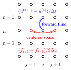
A forward time centered space difference scheme might spring to mind
as a natural one, illustrated in Fig.&nbsp;<a href="chap7.xml#fluidFTCSl">7.4</a>. 

<div class="p"><!----></div>
<a id="tth_fIg7.4">
</a>   <img src="figures/fluidFTCS.png" alt="figures/fluidFTCS.png" /><a id="fluidFTCS">
</a>
  
<div style="text-align:center">Figure 7.4: Forward derivative in Time (<math xmlns="http://www.w3.org/1998/Math/MathML">
<mrow><mi>n</mi></mrow></math>) and Centered in Space (<math xmlns="http://www.w3.org/1998/Math/MathML">
<mrow><mi>j</mi></mrow></math>) (FTCS)
    finite differences give rise to an unstable scheme for hyperbolic problems.<a id="fluidFTCSl">
</a></div> 

<div class="p"><!----></div>
 For stability<a 
id="hyperbolic_stability73455"></a> 
analysis<a 
id="stability_hyperbolic73456"></a> purposes, we can suppose that
we are using the new representation (in other words <math xmlns="http://www.w3.org/1998/Math/MathML">
<mrow><mi>u</mi></mrow></math> stands for
each <math xmlns="http://www.w3.org/1998/Math/MathML">
<mrow><mi>q</mi></mrow></math> which we can consider separately in scalar equations).
But we
don't actually do the transformation to that new representation when
implementing the scheme (only when analysing its stability). The first
time through we'll do things explicitly but then take short cuts
thereafter not bringing <math xmlns="http://www.w3.org/1998/Math/MathML">
<mrow><mi>q</mi></mrow></math> in explicitly. We write
out the difference equation as
<a id="FTCShyper">
</a><br />
<table width="100%"><tr><td align="center">
    <math xmlns="http://www.w3.org/1998/Math/MathML">
    <mstyle displaystyle="true"><mrow>
<msubsup><mrow><mi mathvariant="bold">u</mi></mrow><mrow><mi>j</mi> </mrow>
<mrow><mo stretchy="false">(</mo><mi>n</mi><mo>+</mo><mn>1</mn><mo stretchy="false">)</mo></mrow></msubsup>
<mo>-</mo>
<msubsup><mrow><mi mathvariant="bold">u</mi></mrow><mrow><mi>j</mi> </mrow>
<mrow><mo stretchy="false">(</mo><mi>n</mi><mo stretchy="false">)</mo></mrow></msubsup>
<mo>=</mo><mo>-</mo>
<mfrac><mrow><mi mathvariant="italic">&Delta;</mi><mi>t</mi></mrow>
<mrow><mn>2</mn><mi mathvariant="italic">&Delta;</mi><mi>x</mi></mrow>
</mfrac>
<mo stretchy="false">(</mo>
<msubsup><mrow><mi mathvariant="bold">f</mi></mrow><mrow><mi>j</mi><mo>+</mo><mn>1</mn> </mrow>
<mrow><mo stretchy="false">(</mo><mi>n</mi><mo stretchy="false">)</mo></mrow></msubsup>
<mo>-</mo>
<msubsup><mrow><mi mathvariant="bold">f</mi></mrow><mrow><mi>j</mi><mo>-</mo><mn>1</mn> </mrow>
<mrow><mo stretchy="false">(</mo><mi>n</mi><mo stretchy="false">)</mo></mrow></msubsup>
<mo stretchy="false">)</mo><mo>=</mo><mo>-</mo>
<mfrac><mrow><mi mathvariant="italic">&Delta;</mi><mi>t</mi></mrow>
<mrow><mn>2</mn><mi mathvariant="italic">&Delta;</mi><mi>x</mi></mrow>
</mfrac>
<mi mathvariant="bold">J</mi><mo stretchy="false">(</mo>
<msubsup><mrow><mi mathvariant="bold">u</mi></mrow><mrow><mi>j</mi><mo>+</mo><mn>1</mn> </mrow>
<mrow><mo stretchy="false">(</mo><mi>n</mi><mo stretchy="false">)</mo></mrow></msubsup>
<mo>-</mo>
<msubsup><mrow><mi mathvariant="bold">u</mi></mrow><mrow><mi>j</mi><mo>-</mo><mn>1</mn> </mrow>
<mrow><mo stretchy="false">(</mo><mi>n</mi><mo stretchy="false">)</mo></mrow></msubsup>
<mo stretchy="false">)</mo><mo>,</mo></mrow>
    </mstyle></math></td><td width="1">
    <math xmlns="http://www.w3.org/1998/Math/MathML">
    <mstyle displaystyle="true"><mrow><mo stretchy="false">(</mo><mn>7</mn><mo>.</mo><mn>22</mn><mo stretchy="false">)</mo></mrow>
    </mstyle></math>
</td></tr></table>


which in the new representation is 
<a id="FTCShyperalt">
</a><br />
<table width="100%"><tr><td align="center">
    <math xmlns="http://www.w3.org/1998/Math/MathML">
    <mstyle displaystyle="true"><mrow>
<msubsup><mrow><mi>q</mi></mrow><mrow><mi>j</mi> </mrow>
<mrow><mo stretchy="false">(</mo><mi>n</mi><mo>+</mo><mn>1</mn><mo stretchy="false">)</mo></mrow></msubsup>
<mo>-</mo>
<msubsup><mrow><mi>q</mi></mrow><mrow><mi>j</mi> </mrow>
<mrow><mo stretchy="false">(</mo><mi>n</mi><mo stretchy="false">)</mo></mrow></msubsup>
<mo>=</mo><mo>-</mo>
<mfrac><mrow><mi mathvariant="italic">&Delta;</mi><mi>t</mi></mrow>
<mrow><mn>2</mn><mi mathvariant="italic">&Delta;</mi><mi>x</mi></mrow>
</mfrac>
<mi mathvariant="italic">&lambda;</mi><mo stretchy="false">(</mo>
<msubsup><mrow><mi>q</mi></mrow><mrow><mi>j</mi><mo>+</mo><mn>1</mn> </mrow>
<mrow><mo stretchy="false">(</mo><mi>n</mi><mo stretchy="false">)</mo></mrow></msubsup>
<mo>-</mo>
<msubsup><mrow><mi>q</mi></mrow><mrow><mi>j</mi><mo>-</mo><mn>1</mn> </mrow>
<mrow><mo stretchy="false">(</mo><mi>n</mi><mo stretchy="false">)</mo></mrow></msubsup>
<mo stretchy="false">)</mo></mrow>
    </mstyle></math></td><td width="1">
    <math xmlns="http://www.w3.org/1998/Math/MathML">
    <mstyle displaystyle="true"><mrow><mo stretchy="false">(</mo><mn>7</mn><mo>.</mo><mn>23</mn><mo stretchy="false">)</mo></mrow>
    </mstyle></math>
</td></tr></table>


and consider a single spatial Fourier mode of <math xmlns="http://www.w3.org/1998/Math/MathML">
<mrow><mi>u</mi></mrow></math> and <math xmlns="http://www.w3.org/1998/Math/MathML">
<mrow><mi>f</mi></mrow></math> and hence of <math xmlns="http://www.w3.org/1998/Math/MathML">
<mrow><mi>q</mi></mrow></math>
<a id="uFourier">
</a><br />
<table width="100%"><tr><td align="center">
    <math xmlns="http://www.w3.org/1998/Math/MathML">
    <mstyle displaystyle="true"><mrow>
<msub><mrow><mi>q</mi></mrow><mrow><mi>j</mi></mrow>
</msub>
<mo>=</mo><mi>q</mi><mi>exp</mi><mo stretchy="false">(</mo>
<msub><mrow><mi mathvariant="italic">ik</mi></mrow><mrow><mi>x</mi></mrow>
</msub>
<mi>j</mi><mi mathvariant="italic">&Delta;</mi><mi>x</mi><mo stretchy="false">)</mo><mo>,</mo><mi>&emsp;&emsp;&emsp;&emsp;&emsp;&emsp;</mi>
<msub><mrow><mi>f</mi></mrow><mrow><mi>j</mi></mrow>
</msub>
<mo>=</mo><mi>f</mi><mi>exp</mi><mo stretchy="false">(</mo>
<msub><mrow><mi mathvariant="italic">ik</mi></mrow><mrow><mi>x</mi></mrow>
</msub>
<mi>j</mi><mi mathvariant="italic">&Delta;</mi><mi>x</mi><mo stretchy="false">)</mo><mo>.</mo></mrow>
    </mstyle></math></td><td width="1">
    <math xmlns="http://www.w3.org/1998/Math/MathML">
    <mstyle displaystyle="true"><mrow><mo stretchy="false">(</mo><mn>7</mn><mo>.</mo><mn>24</mn><mo stretchy="false">)</mo></mrow>
    </mstyle></math>
</td></tr></table>


Substituting for the spatial dependence, the advancing equation becomes
<a id="FTCShyperIt">
</a><br />
<table width="100%"><tr><td align="center">
    <math xmlns="http://www.w3.org/1998/Math/MathML">
    <mstyle displaystyle="true"><mrow>
<msubsup><mrow><mi>q</mi></mrow><mrow><mi>j</mi> </mrow>
<mrow><mo stretchy="false">(</mo><mi>n</mi><mo>+</mo><mn>1</mn><mo stretchy="false">)</mo></mrow></msubsup>
<mo>=</mo><mo stretchy="false">[</mo><mn>1</mn><mo>-</mo>
<mfrac><mrow><mi mathvariant="italic">&Delta;</mi><mi>t</mi><mi mathvariant="italic">&lambda;</mi></mrow>
<mrow><mn>2</mn><mi mathvariant="italic">&Delta;</mi><mi>x</mi></mrow>
</mfrac>
<mo stretchy="false">(</mo>
<msup><mrow><mi fontstyle="normal">e</mi></mrow><mrow>
<msub><mrow><mi mathvariant="italic">ik</mi></mrow><mrow><mi>x</mi></mrow>
</msub>
<mi mathvariant="italic">&Delta;</mi><mi>x</mi></mrow>
</msup>
<mo>-</mo>
<msup><mrow><mi fontstyle="normal">e</mi></mrow><mrow><mo>-</mo>
<msub><mrow><mi mathvariant="italic">ik</mi></mrow><mrow><mi>x</mi></mrow>
</msub>
<mi mathvariant="italic">&Delta;</mi><mi>x</mi></mrow>
</msup>
<mo stretchy="false">)</mo><mo stretchy="false">]</mo>
<msubsup><mrow><mi>q</mi></mrow><mrow><mi>j</mi> </mrow>
<mrow><mo stretchy="false">(</mo><mi>n</mi><mo stretchy="false">)</mo></mrow></msubsup>
<mo>=</mo><mo stretchy="false">[</mo><mn>1</mn><mo>-</mo><mi>i</mi>
<mfrac><mrow><mi mathvariant="italic">&Delta;</mi><mi>t</mi><mi mathvariant="italic">&lambda;</mi></mrow>
<mrow><mi mathvariant="italic">&Delta;</mi><mi>x</mi></mrow>
</mfrac>
<mi>sin</mi><mo stretchy="false">(</mo>
<msub><mrow><mi>k</mi></mrow><mrow><mi>x</mi></mrow>
</msub>
<mi mathvariant="italic">&Delta;</mi><mi>x</mi><mo stretchy="false">)</mo><mo stretchy="false">]</mo>
<msubsup><mrow><mi>q</mi></mrow><mrow><mi>j</mi> </mrow>
<mrow><mo stretchy="false">(</mo><mi>n</mi><mo stretchy="false">)</mo></mrow></msubsup>
<mo>.</mo></mrow>
    </mstyle></math></td><td width="1">
    <math xmlns="http://www.w3.org/1998/Math/MathML">
    <mstyle displaystyle="true"><mrow><mo stretchy="false">(</mo><mn>7</mn><mo>.</mo><mn>25</mn><mo stretchy="false">)</mo></mrow>
    </mstyle></math>
</td></tr></table>


Now we see immediately that the temporal amplification factor is
<a id="FTCShyperamp">
</a><br />
<table width="100%"><tr><td align="center">
    <math xmlns="http://www.w3.org/1998/Math/MathML">
    <mstyle displaystyle="true"><mrow><mi>A</mi><mo>=</mo><mn>1</mn><mo>-</mo><mi>i</mi>
<mfrac><mrow><mi mathvariant="italic">&Delta;</mi><mi>t</mi><mi mathvariant="italic">&lambda;</mi></mrow>
<mrow><mi mathvariant="italic">&Delta;</mi><mi>x</mi></mrow>
</mfrac>
<mi>sin</mi><mo stretchy="false">(</mo>
<msub><mrow><mi>k</mi></mrow><mrow><mi>x</mi></mrow>
</msub>
<mi mathvariant="italic">&Delta;</mi><mi>x</mi><mo stretchy="false">)</mo><mo>.</mo></mrow>
    </mstyle></math></td><td width="1">
    <math xmlns="http://www.w3.org/1998/Math/MathML">
    <mstyle displaystyle="true"><mrow><mo stretchy="false">(</mo><mn>7</mn><mo>.</mo><mn>26</mn><mo stretchy="false">)</mo></mrow>
    </mstyle></math>
</td></tr></table>


Because the second term is imaginary, the magnitude of the
amplification factor<a 
id="amplification_factor73457"></a> is always greater
than 1, regardless of the (real) value of <math xmlns="http://www.w3.org/1998/Math/MathML">
<mrow><mi mathvariant="italic">&lambda;</mi></mrow></math>. All modes are
unstable, growing with time!  FTCS does not work for hyperbolic
equations.

<div class="p"><!----></div>
     <a id="tth_sEc7.3.2"></a><h3>
7.3.2&nbsp;&nbsp;Lax-Friedrichs and the CFL condition</h3>

<div class="p"><!----></div>
<a 
id="Lax-Friedrichs_method73458"></a>One tiny change works to stabilize the scheme. That is to replace
<math xmlns="http://www.w3.org/1998/Math/MathML">
<mrow>
<msubsup><mrow><mi>u</mi></mrow><mrow><mi>j</mi> </mrow>
<mrow><mo stretchy="false">(</mo><mi>n</mi><mo stretchy="false">)</mo></mrow></msubsup>
</mrow></math> on the left hand side of eq.&nbsp;(<a href="chap7.xml#FTCShyper">7.22</a>) with
<math xmlns="http://www.w3.org/1998/Math/MathML">
<mrow><mo stretchy="false">(</mo>
<msubsup><mrow><mi>u</mi></mrow><mrow><mi>j</mi><mo>-</mo><mn>1</mn> </mrow>
<mrow><mo stretchy="false">(</mo><mi>n</mi><mo stretchy="false">)</mo></mrow></msubsup>
<mo>+</mo>
<msubsup><mrow><mi>u</mi></mrow><mrow><mi>j</mi><mo>+</mo><mn>1</mn> </mrow>
<mrow><mo stretchy="false">(</mo><mi>n</mi><mo stretchy="false">)</mo></mrow></msubsup>
<mo stretchy="false">)</mo><mo stretchy="false">/</mo><mn>2</mn></mrow></math>, as illustrated in Fig.&nbsp;<a href="chap7.xml#LaxFried">7.5</a>.

<div class="p"><!----></div>
<a id="tth_fIg7.5">
</a>   <img src="figures/LaxFriedrichs.png" alt="figures/LaxFriedrichs.png" /><a id="LaxFriedrichs">
</a>
  
<div style="text-align:center">Figure 7.5: Forward derivative in Time (<math xmlns="http://www.w3.org/1998/Math/MathML">
<mrow><mi>n</mi></mrow></math>) but from the mean of the
    adjacent points  and Centered in Space (<math xmlns="http://www.w3.org/1998/Math/MathML">
<mrow><mi>j</mi></mrow></math>) is the Lax Friedrichs 
    finite difference scheme, which is stable provided <math xmlns="http://www.w3.org/1998/Math/MathML">
<mrow><mi mathvariant="italic">&Delta;</mi><mi>t</mi><mo>&le;</mo><mi mathvariant="italic">&Delta;</mi><mi>x</mi><mo stretchy="false">/</mo><mo stretchy="false">&verbar;</mo><mi mathvariant="italic">&lambda;</mi><mo stretchy="false">&verbar;</mo></mrow></math>.<a id="LaxFried">
</a></div> 

<div class="p"><!----></div>
 This is then called the
Lax-Friedrichs method. 
<a id="LaxFriedrichsl">
</a><br />
<table width="100%"><tr><td align="center">
    <math xmlns="http://www.w3.org/1998/Math/MathML">
    <mstyle displaystyle="true"><mrow>
<msubsup><mrow><mi mathvariant="bold">u</mi></mrow><mrow><mi>j</mi> </mrow>
<mrow><mo stretchy="false">(</mo><mi>n</mi><mo>+</mo><mn>1</mn><mo stretchy="false">)</mo></mrow></msubsup>
<mo>-</mo><mo stretchy="false">(</mo>
<msubsup><mrow><mi mathvariant="bold">u</mi></mrow><mrow><mi>j</mi><mo>-</mo><mn>1</mn> </mrow>
<mrow><mo stretchy="false">(</mo><mi>n</mi><mo stretchy="false">)</mo></mrow></msubsup>
<mo>+</mo>
<msubsup><mrow><mi mathvariant="bold">u</mi></mrow><mrow><mi>j</mi><mo>+</mo><mn>1</mn> </mrow>
<mrow><mo stretchy="false">(</mo><mi>n</mi><mo stretchy="false">)</mo></mrow></msubsup>
<mo stretchy="false">)</mo><mo stretchy="false">/</mo><mn>2</mn><mo>=</mo><mo>-</mo>
<mfrac><mrow><mi mathvariant="italic">&Delta;</mi><mi>t</mi></mrow>
<mrow><mn>2</mn><mi mathvariant="italic">&Delta;</mi><mi>x</mi></mrow>
</mfrac>
<mo stretchy="false">(</mo>
<msubsup><mrow><mi mathvariant="bold">f</mi></mrow><mrow><mi>j</mi><mo>+</mo><mn>1</mn> </mrow>
<mrow><mo stretchy="false">(</mo><mi>n</mi><mo stretchy="false">)</mo></mrow></msubsup>
<mo>-</mo>
<msubsup><mrow><mi mathvariant="bold">f</mi></mrow><mrow><mi>j</mi><mo>-</mo><mn>1</mn> </mrow>
<mrow><mo stretchy="false">(</mo><mi>n</mi><mo stretchy="false">)</mo></mrow></msubsup>
<mo stretchy="false">)</mo><mo>=</mo><mo>-</mo>
<mfrac><mrow><mi mathvariant="italic">&Delta;</mi><mi>t</mi></mrow>
<mrow><mn>2</mn><mi mathvariant="italic">&Delta;</mi><mi>x</mi></mrow>
</mfrac>
<mi mathvariant="bold">J</mi><mo stretchy="false">(</mo>
<msubsup><mrow><mi mathvariant="bold">u</mi></mrow><mrow><mi>j</mi><mo>+</mo><mn>1</mn> </mrow>
<mrow><mo stretchy="false">(</mo><mi>n</mi><mo stretchy="false">)</mo></mrow></msubsup>
<mo>-</mo>
<msubsup><mrow><mi mathvariant="bold">u</mi></mrow><mrow><mi>j</mi><mo>-</mo><mn>1</mn> </mrow>
<mrow><mo stretchy="false">(</mo><mi>n</mi><mo stretchy="false">)</mo></mrow></msubsup>
<mo stretchy="false">)</mo><mo>.</mo></mrow>
    </mstyle></math></td><td width="1">
    <math xmlns="http://www.w3.org/1998/Math/MathML">
    <mstyle displaystyle="true"><mrow><mo stretchy="false">(</mo><mn>7</mn><mo>.</mo><mn>27</mn><mo stretchy="false">)</mo></mrow>
    </mstyle></math>
</td></tr></table>


The student should verify that replacing <math xmlns="http://www.w3.org/1998/Math/MathML">
<mrow><mi mathvariant="bold">J</mi></mrow></math> with <math xmlns="http://www.w3.org/1998/Math/MathML">
<mrow><mi mathvariant="italic">&lambda;</mi></mrow></math> for
a scalar version of these equations, the resulting
amplification factor<a 
id="amplification_factor73459"></a> is
<a id="LaxFriedrichsamp">
</a><br />
<table width="100%"><tr><td align="center">
    <math xmlns="http://www.w3.org/1998/Math/MathML">
    <mstyle displaystyle="true"><mrow><mi>A</mi><mo>=</mo><mi>cos</mi><mo stretchy="false">(</mo>
<msub><mrow><mi>k</mi></mrow><mrow><mi>x</mi></mrow>
</msub>
<mi mathvariant="italic">&Delta;</mi><mi>x</mi><mo stretchy="false">)</mo><mo>-</mo><mi>i</mi>
<mfrac><mrow><mi mathvariant="italic">&Delta;</mi><mi>t</mi><mi mathvariant="italic">&lambda;</mi></mrow>
<mrow><mi mathvariant="italic">&Delta;</mi><mi>x</mi></mrow>
</mfrac>
<mi>sin</mi><mo stretchy="false">(</mo>
<msub><mrow><mi>k</mi></mrow><mrow><mi>x</mi></mrow>
</msub>
<mi mathvariant="italic">&Delta;</mi><mi>x</mi><mo stretchy="false">)</mo><mo>.</mo></mrow>
    </mstyle></math></td><td width="1">
    <math xmlns="http://www.w3.org/1998/Math/MathML">
    <mstyle displaystyle="true"><mrow><mo stretchy="false">(</mo><mn>7</mn><mo>.</mo><mn>28</mn><mo stretchy="false">)</mo></mrow>
    </mstyle></math>
</td></tr></table>


As <math xmlns="http://www.w3.org/1998/Math/MathML">
<mrow>
<msub><mrow><mi>k</mi></mrow><mrow><mi>x</mi></mrow>
</msub>
</mrow></math> varies, this is the equation of an ellipse in the complex plane. For
stability, this ellipse must be entirely inside the unit circle, which
requires the imaginary coefficient's magnitude to be less than or equal to 1
<a id="CFL">
</a><br />
<table width="100%"><tr><td align="center">
    <math xmlns="http://www.w3.org/1998/Math/MathML">
    <mstyle displaystyle="true"><mrow><mi mathvariant="italic">&Delta;</mi><mi>t</mi><mo>&le;</mo><mi mathvariant="italic">&Delta;</mi><mi>x</mi><mo stretchy="false">/</mo><mo stretchy="false">&verbar;</mo><mi mathvariant="italic">&lambda;</mi><mo stretchy="false">&verbar;</mo><mo>.</mo></mrow>
    </mstyle></math></td><td width="1">
    <math xmlns="http://www.w3.org/1998/Math/MathML">
    <mstyle displaystyle="true"><mrow><mo stretchy="false">(</mo><mn>7</mn><mo>.</mo><mn>29</mn><mo stretchy="false">)</mo></mrow>
    </mstyle></math>
</td></tr></table>


For our fluid example this is <math xmlns="http://www.w3.org/1998/Math/MathML">
<mrow><mi mathvariant="italic">&Delta;</mi><mi>t</mi><mo>&le;</mo><mi mathvariant="italic">&Delta;</mi><mi>x</mi><mo stretchy="false">/</mo><mo stretchy="false">&verbar;</mo><mi>v</mi><mo>&PlusMinus;</mo>
<msub><mrow><mi>c</mi></mrow><mrow><mi>s</mi></mrow>
</msub>
<mo stretchy="false">&verbar;</mo></mrow></math>.
Equation (<a href="chap7.xml#CFL">7.29</a>) is called the
Courant-Friedrichs-Lewy<a 
id="Courant-Friedrichs-Lewy73460"></a><a 
id="CFL___condition73461"></a> (CFL) condition. It applies to essentially all explicit
schemes for hyperbolic equations. It says that <math xmlns="http://www.w3.org/1998/Math/MathML">
<mrow><mi mathvariant="italic">&Delta;</mi><mi>t</mi></mrow></math> must be less
than the time it takes for influence to propagate at the
characteristic speed(s) (given by the eigenvalues of <math xmlns="http://www.w3.org/1998/Math/MathML">
<mrow><mi mathvariant="bold">J</mi></mrow></math>) from
the prior adjacent nodes. If it were greater, then influence from
other nodes, not taken into account in the difference scheme, would
influence the solution.

<div class="p"><!----></div>
     <a id="tth_sEc7.3.3"></a><h3>
7.3.3&nbsp;&nbsp;Lax-Wendroff achieves second order accuracy</h3>

<div class="p"><!----></div>
<a 
id="Lax-Wendroff_method73462"></a>The low order errors of the Lax-Friedrichs scheme make it of little
practical value. It has a substantial level of spurious
<em>numerical diffusion</em><a 
id="numerical___diffusion73463"></a><a 
id="diffusion_numerical73464"></a>
that damps out perturbations that should
not be damped. For example the simple fluid we've used to illustrate
the issues has no physical dissipation, yet for some modes
Lax-Friedrichs gives <math xmlns="http://www.w3.org/1998/Math/MathML">
<mrow><mo stretchy="false">&verbar;</mo><mi>A</mi><mo stretchy="false">&verbar;</mo></mrow></math> substantially less than one. They are
damped.  A better scheme, which is second order in time and still stable, is the
Lax-Wendroff scheme. The advance is implemented in two steps:
<a id="LaxW1">
</a><br />
<table width="100%"><tr><td align="center">
    <math xmlns="http://www.w3.org/1998/Math/MathML">
    <mstyle displaystyle="true"><mrow>
<msubsup><mrow><mi mathvariant="bold">u</mi></mrow><mrow><mi>j</mi><mo>+</mo><mn>1</mn><mo stretchy="false">/</mo><mn>2</mn> </mrow>
<mrow><mo stretchy="false">(</mo><mi>n</mi><mo>+</mo><mn>1</mn><mo stretchy="false">/</mo><mn>2</mn><mo stretchy="false">)</mo></mrow></msubsup>
<mo>=</mo>
<mfrac><mrow><mn>1</mn></mrow>
<mrow><mn>2</mn></mrow>
</mfrac>
<mrow><mo>(</mo>
<msubsup><mrow><mi mathvariant="bold">u</mi></mrow><mrow><mi>j</mi><mo>+</mo><mn>1</mn> </mrow>
<mrow><mo stretchy="false">(</mo><mi>n</mi><mo stretchy="false">)</mo></mrow></msubsup>
<mo>+</mo>
<msubsup><mrow><mi mathvariant="bold">u</mi></mrow><mrow><mi>j</mi> </mrow>
<mrow><mo stretchy="false">(</mo><mi>n</mi><mo stretchy="false">)</mo></mrow></msubsup>
<mo>)</mo></mrow><mo>-</mo>
<mfrac><mrow><mi mathvariant="italic">&Delta;</mi><mi>t</mi></mrow>
<mrow><mn>2</mn><mi mathvariant="italic">&Delta;</mi><mi>x</mi></mrow>
</mfrac>
<mrow><mo>(</mo>
<msubsup><mrow><mi mathvariant="bold">f</mi></mrow><mrow><mi>j</mi><mo>+</mo><mn>1</mn> </mrow>
<mrow><mo stretchy="false">(</mo><mi>n</mi><mo stretchy="false">)</mo></mrow></msubsup>
<mo>-</mo>
<msubsup><mrow><mi mathvariant="bold">f</mi></mrow><mrow><mi>j</mi> </mrow>
<mrow><mo stretchy="false">(</mo><mi>n</mi><mo stretchy="false">)</mo></mrow></msubsup>
<mo>)</mo></mrow></mrow>
    </mstyle></math></td><td width="1">
    <math xmlns="http://www.w3.org/1998/Math/MathML">
    <mstyle displaystyle="true"><mrow><mo stretchy="false">(</mo><mn>7</mn><mo>.</mo><mn>30</mn><mo stretchy="false">)</mo></mrow>
    </mstyle></math>
</td></tr></table>


<a id="LaxW2">
</a><br />
<table width="100%"><tr><td align="center">
    <math xmlns="http://www.w3.org/1998/Math/MathML">
    <mstyle displaystyle="true"><mrow>
<msubsup><mrow><mi mathvariant="bold">u</mi></mrow><mrow><mi>j</mi> </mrow>
<mrow><mo stretchy="false">(</mo><mi>n</mi><mo>+</mo><mn>1</mn><mo stretchy="false">)</mo></mrow></msubsup>
<mo>=</mo>
<msubsup><mrow><mi mathvariant="bold">u</mi></mrow><mrow><mi>j</mi> </mrow>
<mrow><mo stretchy="false">(</mo><mi>n</mi><mo stretchy="false">)</mo></mrow></msubsup>
<mo>-</mo>
<mfrac><mrow><mi mathvariant="italic">&Delta;</mi><mi>t</mi></mrow>
<mrow><mi mathvariant="italic">&Delta;</mi><mi>x</mi></mrow>
</mfrac>
<mrow><mo>(</mo>
<msubsup><mrow><mi mathvariant="bold">f</mi></mrow><mrow><mi>j</mi><mo>+</mo><mn>1</mn><mo stretchy="false">/</mo><mn>2</mn> </mrow>
<mrow><mo stretchy="false">(</mo><mi>n</mi><mo>+</mo><mn>1</mn><mo stretchy="false">/</mo><mn>2</mn><mo stretchy="false">)</mo></mrow></msubsup>
<mo>-</mo>
<msubsup><mrow><mi mathvariant="bold">f</mi></mrow><mrow><mi>j</mi><mo>-</mo><mn>1</mn><mo stretchy="false">/</mo><mn>2</mn> </mrow>
<mrow><mo stretchy="false">(</mo><mi>n</mi><mo>+</mo><mn>1</mn><mo stretchy="false">/</mo><mn>2</mn><mo stretchy="false">)</mo></mrow></msubsup>
<mo>)</mo></mrow><mo>.</mo></mrow>
    </mstyle></math></td><td width="1">
    <math xmlns="http://www.w3.org/1998/Math/MathML">
    <mstyle displaystyle="true"><mrow><mo stretchy="false">(</mo><mn>7</mn><mo>.</mo><mn>31</mn><mo stretchy="false">)</mo></mrow>
    </mstyle></math>
</td></tr></table>


Fig.&nbsp;<a href="chap7.xml#LaxWend">7.6</a> shows the schematic.

<div class="p"><!----></div>
<a id="tth_fIg7.6">
</a>   <img src="figures/LaxWendroff.png" alt="figures/LaxWendroff.png" /><a id="LaxWendroff">
</a>
  
<div style="text-align:center">Figure 7.6: The Lax-Wendroff two-step scheme first (dashed lines)
    generates <math xmlns="http://www.w3.org/1998/Math/MathML">
<mrow><mi>u</mi></mrow></math> and hence <math xmlns="http://www.w3.org/1998/Math/MathML">
<mrow><mi>f</mi></mrow></math> values at the half-time-step <math xmlns="http://www.w3.org/1998/Math/MathML">
<mrow><mi>n</mi><mo>+</mo>
<mfrac><mrow><mn>1</mn></mrow>
<mrow><mn>2</mn></mrow>
</mfrac>
</mrow></math>,
    by a Lax-Friedrichs advance to (<b>X</b>). Then it uses a centered time,
    centered space full step advance based upon <math xmlns="http://www.w3.org/1998/Math/MathML">
<mrow>
<msup><mrow><mi mathvariant="bold">f</mi></mrow><mrow><mo stretchy="false">(</mo><mi>n</mi><mo>+</mo><mn>1</mn><mo stretchy="false">/</mo><mn>2</mn><mo stretchy="false">)</mo></mrow>
</msup>
</mrow></math>,
    from the <math xmlns="http://www.w3.org/1998/Math/MathML">
<mrow>
<msup><mrow><mi mathvariant="bold">u</mi></mrow><mrow><mo stretchy="false">(</mo><mi>n</mi><mo stretchy="false">)</mo></mrow>
</msup>
</mrow></math>.<a id="LaxWend">
</a></div>

<div class="p"><!----></div>
The first step is like a Lax-Friedrichs half-step to the half-way
positions. Then the fluxes are evaluated again, at the half-step
times and positions using the <math xmlns="http://www.w3.org/1998/Math/MathML">
<mrow>
<msup><mrow><mi mathvariant="bold">u</mi></mrow><mrow><mo stretchy="false">(</mo><mi>n</mi><mo>+</mo><mn>1</mn><mo stretchy="false">/</mo><mn>2</mn><mo stretchy="false">)</mo></mrow>
</msup>
</mrow></math> values, to find the
<math xmlns="http://www.w3.org/1998/Math/MathML">
<mrow>
<msup><mrow><mi mathvariant="bold">f</mi></mrow><mrow><mo stretchy="false">(</mo><mi>n</mi><mo>+</mo><mn>1</mn><mo stretchy="false">/</mo><mn>2</mn><mo stretchy="false">)</mo></mrow>
</msup>
</mrow></math>. Those are used in the second step to advance all
the way from <math xmlns="http://www.w3.org/1998/Math/MathML">
<mrow><mi>n</mi></mrow></math> to <math xmlns="http://www.w3.org/1998/Math/MathML">
<mrow><mi>n</mi><mo>+</mo><mn>1</mn></mrow></math> in a properly centered manner.
The amplification factor for the combined step can be shown to be 
<a id="LaxWA">
</a><br />
<table width="100%"><tr><td align="center">
    <math xmlns="http://www.w3.org/1998/Math/MathML">
    <mstyle displaystyle="true"><mrow><mi>A</mi><mo>=</mo><mn>1</mn><mo>-</mo><mi>i</mi>
<mfrac><mrow><mi mathvariant="italic">&Delta;</mi><mi>t</mi><mi mathvariant="italic">&lambda;</mi></mrow>
<mrow><mi mathvariant="italic">&Delta;</mi><mi>x</mi></mrow>
</mfrac>
<mi>sin</mi><mo stretchy="false">(</mo>
<msub><mrow><mi>k</mi></mrow><mrow><mi>x</mi></mrow>
</msub>
<mi mathvariant="italic">&Delta;</mi><mi>x</mi><mo stretchy="false">)</mo><mo>+</mo>
<msup><mrow><mo>(</mo>
<mfrac><mrow><mi mathvariant="italic">&Delta;</mi><mi>t</mi><mi mathvariant="italic">&lambda;</mi></mrow>
<mrow><mi mathvariant="italic">&Delta;</mi><mi>x</mi></mrow>
</mfrac>
<mo>)</mo></mrow><mrow><mn>2</mn></mrow>
</msup>
<mo stretchy="false">[</mo><mi>cos</mi><mo stretchy="false">(</mo>
<msub><mrow><mi>k</mi></mrow><mrow><mi>x</mi></mrow>
</msub>
<mi mathvariant="italic">&Delta;</mi><mi>x</mi><mo stretchy="false">)</mo><mo>-</mo><mn>1</mn><mo stretchy="false">]</mo></mrow>
    </mstyle></math></td><td width="1">
    <math xmlns="http://www.w3.org/1998/Math/MathML">
    <mstyle displaystyle="true"><mrow><mo stretchy="false">(</mo><mn>7</mn><mo>.</mo><mn>32</mn><mo stretchy="false">)</mo></mrow>
    </mstyle></math>
</td></tr></table>


which gives stability if <math xmlns="http://www.w3.org/1998/Math/MathML">
<mrow>
<mfrac><mrow><mi mathvariant="italic">&Delta;</mi><mi>t</mi><mo stretchy="false">&verbar;</mo><mi mathvariant="italic">&lambda;</mi><mo stretchy="false">&verbar;</mo></mrow>
<mrow><mi mathvariant="italic">&Delta;</mi><mi>x</mi></mrow>
</mfrac>
<mo>&le;</mo><mn>1</mn></mrow></math>: the CFL
condition, the same as before.

<div class="p"><!----></div>
There are several other schemes in regular use for solving first order
hyperbolic problems to second order
accuracy<a 
id="second-order_accuracy73465"></a>. They practically all use
multi-step approaches like the Lax-Wendroff method.

<div class="p"><!----></div>

<h2>Worked Example. Stability of Lax-Wendroff scheme.</h2>

<div class="p"><!----></div>
Derive the amplification factor<a 
id="Lax-Wendroff_method73466"></a> for the
Lax-Wendroff scheme and verify the stability condition <math xmlns="http://www.w3.org/1998/Math/MathML">
<mrow>
<mfrac><mrow><mi mathvariant="italic">&Delta;</mi><mi>t</mi><mo stretchy="false">&verbar;</mo><mi mathvariant="italic">&lambda;</mi><mo stretchy="false">&verbar;</mo></mrow>
<mrow><mi mathvariant="italic">&Delta;</mi><mi>x</mi></mrow>
</mfrac>
<mo>&le;</mo><mn>1</mn></mrow></math>.  
<div class="p"><!----></div>
<br />Start with the formula for the first time half-step: eq.&nbsp;(<a href="chap7.xml#LaxW1">7.30</a>). For stability analysis (but not in implementing an
actual numerical scheme), approximate the Jacobian matrix locally as
uniform, and substitute <math xmlns="http://www.w3.org/1998/Math/MathML">
<mrow><mi mathvariant="bold">f</mi><mo>=</mo><mi mathvariant="bold">J</mi><mi mathvariant="bold">u</mi></mrow></math> at all the required
mesh positions,
deriving
<a id="wk7eq1">
</a><br />
<table width="100%"><tr><td align="center">
    <math xmlns="http://www.w3.org/1998/Math/MathML">
    <mstyle displaystyle="true"><mrow>
<mtable>
<mtr><mtd columnalign="right"><mrow>
<msubsup><mrow><mi mathvariant="bold">u</mi></mrow><mrow><mi>j</mi><mo>+</mo><mn>1</mn><mo stretchy="false">/</mo><mn>2</mn> </mrow>
<mrow><mo stretchy="false">(</mo><mi>n</mi><mo>+</mo><mn>1</mn><mo stretchy="false">/</mo><mn>2</mn><mo stretchy="false">)</mo></mrow></msubsup>
</mrow></mtd><mtd columnalign="left"><mrow><mo>=</mo>
<mfrac><mrow><mn>1</mn></mrow>
<mrow><mn>2</mn></mrow>
</mfrac>
<mrow><mo>(</mo>
<msubsup><mrow><mi mathvariant="bold">u</mi></mrow><mrow><mi>j</mi><mo>+</mo><mn>1</mn> </mrow>
<mrow><mo stretchy="false">(</mo><mi>n</mi><mo stretchy="false">)</mo></mrow></msubsup>
<mo>+</mo>
<msubsup><mrow><mi mathvariant="bold">u</mi></mrow><mrow><mi>j</mi> </mrow>
<mrow><mo stretchy="false">(</mo><mi>n</mi><mo stretchy="false">)</mo></mrow></msubsup>
<mo>)</mo></mrow><mo>-</mo>
<mfrac><mrow><mi mathvariant="italic">&Delta;</mi><mi>t</mi></mrow>
<mrow><mn>2</mn><mi mathvariant="italic">&Delta;</mi><mi>x</mi></mrow>
</mfrac>
<mi mathvariant="bold">J</mi><mrow><mo>(</mo>
<msubsup><mrow><mi mathvariant="bold">u</mi></mrow><mrow><mi>j</mi><mo>+</mo><mn>1</mn> </mrow>
<mrow><mo stretchy="false">(</mo><mi>n</mi><mo stretchy="false">)</mo></mrow></msubsup>
<mo>-</mo>
<msubsup><mrow><mi mathvariant="bold">u</mi></mrow><mrow><mi>j</mi> </mrow>
<mrow><mo stretchy="false">(</mo><mi>n</mi><mo stretchy="false">)</mo></mrow></msubsup>
<mo>)</mo></mrow></mrow></mtd></mtr>
<mtr><mtd columnalign="right"><mrow></mrow></mtd><mtd columnalign="left"><mrow><mo>=</mo>
<mfrac><mrow><mn>1</mn></mrow>
<mrow><mn>2</mn></mrow>
</mfrac>
<mrow><mo>[</mo><mo stretchy="false">(</mo><mi mathvariant="bold">I</mi><mo>-</mo>
<mfrac><mrow><mi mathvariant="italic">&Delta;</mi><mi>t</mi></mrow>
<mrow><mi mathvariant="italic">&Delta;</mi><mi>x</mi></mrow>
</mfrac>
<mi mathvariant="bold">J</mi><mo stretchy="false">)</mo>
<msubsup><mrow><mi mathvariant="bold">u</mi></mrow><mrow><mi>j</mi><mo>+</mo><mn>1</mn> </mrow>
<mrow><mo stretchy="false">(</mo><mi>n</mi><mo stretchy="false">)</mo></mrow></msubsup>
<mo>+</mo><mo stretchy="false">(</mo><mi mathvariant="bold">I</mi><mo>+</mo>
<mfrac><mrow><mi mathvariant="italic">&Delta;</mi><mi>t</mi></mrow>
<mrow><mi mathvariant="italic">&Delta;</mi><mi>x</mi></mrow>
</mfrac>
<mi mathvariant="bold">J</mi><mo stretchy="false">)</mo>
<msubsup><mrow><mi mathvariant="bold">u</mi></mrow><mrow><mi>j</mi> </mrow>
<mrow><mo stretchy="false">(</mo><mi>n</mi><mo stretchy="false">)</mo></mrow></msubsup>
<mo>]</mo></mrow><mo>.</mo></mrow></mtd></mtr></mtable>

</mrow>
    </mstyle></math></td><td width="1">
    <math xmlns="http://www.w3.org/1998/Math/MathML">
    <mstyle displaystyle="true"><mrow><mo stretchy="false">(</mo><mn>7</mn><mo>.</mo><mn>33</mn><mo stretchy="false">)</mo></mrow>
    </mstyle></math>
</td></tr></table>


Similarly, the second half-step can be written:
<a id="wk7eq0">
</a><br />
<table width="100%"><tr><td align="center">
    <math xmlns="http://www.w3.org/1998/Math/MathML">
    <mstyle displaystyle="true"><mrow>
<msubsup><mrow><mi mathvariant="bold">u</mi></mrow><mrow><mi>j</mi> </mrow>
<mrow><mo stretchy="false">(</mo><mi>n</mi><mo>+</mo><mn>1</mn><mo stretchy="false">)</mo></mrow></msubsup>
<mo>=</mo>
<msubsup><mrow><mi mathvariant="bold">u</mi></mrow><mrow><mi>j</mi> </mrow>
<mrow><mo stretchy="false">(</mo><mi>n</mi><mo stretchy="false">)</mo></mrow></msubsup>
<mo>-</mo>
<mfrac><mrow><mi mathvariant="italic">&Delta;</mi><mi>t</mi></mrow>
<mrow><mi mathvariant="italic">&Delta;</mi><mi>x</mi></mrow>
</mfrac>
<mi mathvariant="bold">J</mi><mrow><mo>(</mo>
<msubsup><mrow><mi mathvariant="bold">u</mi></mrow><mrow><mi>j</mi><mo>+</mo><mn>1</mn><mo stretchy="false">/</mo><mn>2</mn> </mrow>
<mrow><mo stretchy="false">(</mo><mi>n</mi><mo>+</mo><mn>1</mn><mo stretchy="false">/</mo><mn>2</mn><mo stretchy="false">)</mo></mrow></msubsup>
<mo>-</mo>
<msubsup><mrow><mi mathvariant="bold">u</mi></mrow><mrow><mi>j</mi><mo>-</mo><mn>1</mn><mo stretchy="false">/</mo><mn>2</mn> </mrow>
<mrow><mo stretchy="false">(</mo><mi>n</mi><mo>+</mo><mn>1</mn><mo stretchy="false">/</mo><mn>2</mn><mo stretchy="false">)</mo></mrow></msubsup>
<mo>)</mo></mrow><mo>.</mo></mrow>
    </mstyle></math></td><td width="1">
    <math xmlns="http://www.w3.org/1998/Math/MathML">
    <mstyle displaystyle="true"><mrow><mo stretchy="false">(</mo><mn>7</mn><mo>.</mo><mn>34</mn><mo stretchy="false">)</mo></mrow>
    </mstyle></math>
</td></tr></table>


Substitute for the half-step values from eq.&nbsp;(<a href="chap7.xml#wk7eq1">7.33</a>) to find:
<a id="wk7eq2">
</a><br />
<table width="100%"><tr><td align="center">
    <math xmlns="http://www.w3.org/1998/Math/MathML">
    <mstyle displaystyle="true"><mrow>
<mtable displaystyle="true" align="right" width="80%">
<mtr><mtd columnalign="right" columnspan="1"><mrow>
<msubsup><mrow><mi mathvariant="bold">u</mi></mrow><mrow><mi>j</mi> </mrow>
<mrow><mo stretchy="false">(</mo><mi>n</mi><mo>+</mo><mn>1</mn><mo stretchy="false">)</mo></mrow></msubsup>
<mo>-</mo>
<msubsup><mrow><mi mathvariant="bold">u</mi></mrow><mrow><mi>j</mi> </mrow>
<mrow><mo stretchy="false">(</mo><mi>n</mi><mo stretchy="false">)</mo></mrow></msubsup>
</mrow>
</mtd><mtd columnalign="left">
<mrow><mo>=</mo></mrow>
</mtd><mtd columnalign="left">
<mrow><mo>-</mo>
<mfrac><mrow><mi mathvariant="italic">&Delta;</mi><mi>t</mi></mrow>
<mrow><mn>2</mn><mi mathvariant="italic">&Delta;</mi><mi>x</mi></mrow>
</mfrac>
<mi mathvariant="bold">J</mi><mrow><mo>[</mo><mo stretchy="false">(</mo><mi mathvariant="bold">I</mi><mo>-</mo>
<mfrac><mrow><mi mathvariant="italic">&Delta;</mi><mi>t</mi></mrow>
<mrow><mi mathvariant="italic">&Delta;</mi><mi>x</mi></mrow>
</mfrac>
<mi mathvariant="bold">J</mi><mo stretchy="false">)</mo>
<msubsup><mrow><mi mathvariant="bold">u</mi></mrow><mrow><mi>j</mi><mo>+</mo><mn>1</mn> </mrow>
<mrow><mo stretchy="false">(</mo><mi>n</mi><mo stretchy="false">)</mo></mrow></msubsup>
<mo>+</mo><mo stretchy="false">(</mo><mi mathvariant="bold">I</mi><mo>+</mo>
<mfrac><mrow><mi mathvariant="italic">&Delta;</mi><mi>t</mi></mrow>
<mrow><mi mathvariant="italic">&Delta;</mi><mi>x</mi></mrow>
</mfrac>
<mi mathvariant="bold">J</mi><mo stretchy="false">)</mo>
<msubsup><mrow><mi mathvariant="bold">u</mi></mrow><mrow><mi>j</mi> </mrow>
<mrow><mo stretchy="false">(</mo><mi>n</mi><mo stretchy="false">)</mo></mrow></msubsup>
<mo> </mo></mrow></mrow>
</mtd></mtr>
<mtr><mtd columnalign="right" columnspan="1"><mrow></mrow>
</mtd><mtd columnalign="left">
<mrow></mrow>
</mtd><mtd columnalign="left">
<mrow><mi>&emsp;&emsp;&emsp;&emsp;&emsp;&emsp;</mi><mi>&emsp;&emsp;&emsp;&emsp;&emsp;&emsp;</mi><mrow><mo> </mo><mo>-</mo><mo stretchy="false">(</mo><mi mathvariant="bold">I</mi><mo>-</mo>
<mfrac><mrow><mi mathvariant="italic">&Delta;</mi><mi>t</mi></mrow>
<mrow><mi mathvariant="italic">&Delta;</mi><mi>x</mi></mrow>
</mfrac>
<mi mathvariant="bold">J</mi><mo stretchy="false">)</mo>
<msubsup><mrow><mi mathvariant="bold">u</mi></mrow><mrow><mi>j</mi> </mrow>
<mrow><mo stretchy="false">(</mo><mi>n</mi><mo stretchy="false">)</mo></mrow></msubsup>
<mo>-</mo><mo stretchy="false">(</mo><mi mathvariant="bold">I</mi><mo>+</mo>
<mfrac><mrow><mi mathvariant="italic">&Delta;</mi><mi>t</mi></mrow>
<mrow><mi mathvariant="italic">&Delta;</mi><mi>x</mi></mrow>
</mfrac>
<mi mathvariant="bold">J</mi><mo stretchy="false">)</mo>
<msubsup><mrow><mi mathvariant="bold">u</mi></mrow><mrow><mi>j</mi><mo>-</mo><mn>1</mn> </mrow>
<mrow><mo stretchy="false">(</mo><mi>n</mi><mo stretchy="false">)</mo></mrow></msubsup>
<mo>]</mo></mrow></mrow>
</mtd><mtd columnalign="right">&emsp;&emsp;&emsp;&emsp;&emsp;&emsp;<mo stretchy="false">(</mo><mn>7</mn><mo>.</mo><mn>35</mn><mo stretchy="false">)</mo></mtd></mtr>
<mtr><mtd columnalign="right" columnspan="1"><mrow></mrow>
</mtd><mtd columnalign="left">
<mrow><mo>=</mo></mrow>
</mtd><mtd columnalign="left">
<mrow><mo>-</mo>
<mfrac><mrow><mi mathvariant="italic">&Delta;</mi><mi>t</mi></mrow>
<mrow><mn>2</mn><mi mathvariant="italic">&Delta;</mi><mi>x</mi></mrow>
</mfrac>
<mi mathvariant="bold">J</mi><mrow><mo>[</mo><mo stretchy="false">(</mo>
<msubsup><mrow><mi mathvariant="bold">u</mi></mrow><mrow><mi>j</mi><mo>+</mo><mn>1</mn> </mrow>
<mrow><mo stretchy="false">(</mo><mi>n</mi><mo stretchy="false">)</mo></mrow></msubsup>
<mo>-</mo>
<msubsup><mrow><mi mathvariant="bold">u</mi></mrow><mrow><mi>j</mi><mo>-</mo><mn>1</mn> </mrow>
<mrow><mo stretchy="false">(</mo><mi>n</mi><mo stretchy="false">)</mo></mrow></msubsup>
<mo stretchy="false">)</mo><mo>-</mo>
<mfrac><mrow><mi mathvariant="italic">&Delta;</mi><mi>t</mi></mrow>
<mrow><mi mathvariant="italic">&Delta;</mi><mi>x</mi></mrow>
</mfrac>
<mi mathvariant="bold">J</mi><mo stretchy="false">(</mo>
<msubsup><mrow><mi mathvariant="bold">u</mi></mrow><mrow><mi>j</mi><mo>+</mo><mn>1</mn> </mrow>
<mrow><mo stretchy="false">(</mo><mi>n</mi><mo stretchy="false">)</mo></mrow></msubsup>
<mo>-</mo><mn>2</mn>
<msubsup><mrow><mi mathvariant="bold">u</mi></mrow><mrow><mi>j</mi> </mrow>
<mrow><mo stretchy="false">(</mo><mi>n</mi><mo stretchy="false">)</mo></mrow></msubsup>
<mo>+</mo>
<msubsup><mrow><mi mathvariant="bold">u</mi></mrow><mrow><mi>j</mi><mo>-</mo><mn>1</mn> </mrow>
<mrow><mo stretchy="false">(</mo><mi>n</mi><mo stretchy="false">)</mo></mrow></msubsup>
<mo stretchy="false">)</mo><mo>]</mo></mrow><mo>.</mo></mrow>
</mtd></mtr>
</mtable>
</mrow>
    </mstyle></math>
</td></tr></table>
<br />

Now we consider an eigenmode of <math xmlns="http://www.w3.org/1998/Math/MathML">
<mrow><mi mathvariant="bold">J</mi></mrow></math>, so we can substitute
the eigenvalue <math xmlns="http://www.w3.org/1998/Math/MathML">
<mrow><mi mathvariant="italic">&lambda;</mi></mrow></math> for <math xmlns="http://www.w3.org/1998/Math/MathML">
<mrow><mi mathvariant="bold">J</mi></mrow></math>, everywhere in the above expression.
And we consider a spatial Fourier mode, for which <math xmlns="http://www.w3.org/1998/Math/MathML">
<mrow>
<msub><mrow><mi mathvariant="bold">u</mi></mrow><mrow><mi>j</mi></mrow>
</msub>
<mo>&prop;</mo>
<msup><mrow><mi fontstyle="normal">e</mi></mrow><mrow>
<msub><mrow><mi mathvariant="italic">ik</mi></mrow><mrow><mi>x</mi></mrow>
</msub>
<mi>j</mi><mi mathvariant="italic">&Delta;</mi><mi>x</mi></mrow>
</msup>
</mrow></math>. The equation can then be written
<a id="wk7eq4">
</a><br />
<table width="100%"><tr><td align="center">
    <math xmlns="http://www.w3.org/1998/Math/MathML">
    <mstyle displaystyle="true"><mrow>
<msubsup><mrow><mi mathvariant="bold">u</mi></mrow><mrow><mi>j</mi> </mrow>
<mrow><mo stretchy="false">(</mo><mi>n</mi><mo>+</mo><mn>1</mn><mo stretchy="false">)</mo></mrow></msubsup>
<mo>-</mo>
<msubsup><mrow><mi mathvariant="bold">u</mi></mrow><mrow><mi>j</mi> </mrow>
<mrow><mo stretchy="false">(</mo><mi>n</mi><mo stretchy="false">)</mo></mrow></msubsup>
<mo>=</mo><mo>-</mo>
<mfrac><mrow><mi mathvariant="italic">&Delta;</mi><mi>t</mi></mrow>
<mrow><mn>2</mn><mi mathvariant="italic">&Delta;</mi><mi>x</mi></mrow>
</mfrac>
<mi mathvariant="italic">&lambda;</mi><mrow><mo>[</mo><mo stretchy="false">(</mo>
<msup><mrow><mi fontstyle="normal">e</mi></mrow><mrow>
<msub><mrow><mi mathvariant="italic">ik</mi></mrow><mrow><mi>x</mi></mrow>
</msub>
<mi mathvariant="italic">&Delta;</mi><mi>x</mi></mrow>
</msup>
<mo>-</mo>
<msup><mrow><mi fontstyle="normal">e</mi></mrow><mrow><mo>-</mo>
<msub><mrow><mi mathvariant="italic">ik</mi></mrow><mrow><mi>x</mi></mrow>
</msub>
<mi mathvariant="italic">&Delta;</mi><mi>x</mi></mrow>
</msup>
<mo stretchy="false">)</mo><mo>+</mo>
<mfrac><mrow><mi mathvariant="italic">&Delta;</mi><mi>t</mi></mrow>
<mrow><mi mathvariant="italic">&Delta;</mi><mi>x</mi></mrow>
</mfrac>
<mi mathvariant="italic">&lambda;</mi><mo stretchy="false">(</mo>
<msup><mrow><mi fontstyle="normal">e</mi></mrow><mrow>
<msub><mrow><mi mathvariant="italic">ik</mi></mrow><mrow><mi>x</mi></mrow>
</msub>
<mi mathvariant="italic">&Delta;</mi><mi>x</mi></mrow>
</msup>
<mo>-</mo><mn>2</mn><mo>+</mo>
<msup><mrow><mi fontstyle="normal">e</mi></mrow><mrow><mo>-</mo>
<msub><mrow><mi mathvariant="italic">ik</mi></mrow><mrow><mi>x</mi></mrow>
</msub>
<mi mathvariant="italic">&Delta;</mi><mi>x</mi></mrow>
</msup>
<mo stretchy="false">)</mo><mo>]</mo></mrow>
<msubsup><mrow><mi mathvariant="bold">u</mi></mrow><mrow><mi>j</mi> </mrow>
<mrow><mo stretchy="false">(</mo><mi>n</mi><mo stretchy="false">)</mo></mrow></msubsup>
<mo>,</mo></mrow>
    </mstyle></math></td><td width="1">
    <math xmlns="http://www.w3.org/1998/Math/MathML">
    <mstyle displaystyle="true"><mrow><mo stretchy="false">(</mo><mn>7</mn><mo>.</mo><mn>36</mn><mo stretchy="false">)</mo></mrow>
    </mstyle></math>
</td></tr></table>


or in other words
<a id="wk7eq5">
</a><br />
<table width="100%"><tr><td align="center">
    <math xmlns="http://www.w3.org/1998/Math/MathML">
    <mstyle displaystyle="true"><mrow>
<msubsup><mrow><mi mathvariant="bold">u</mi></mrow><mrow><mi>j</mi> </mrow>
<mrow><mo stretchy="false">(</mo><mi>n</mi><mo>+</mo><mn>1</mn><mo stretchy="false">)</mo></mrow></msubsup>
<mo>=</mo><mrow><mo>{</mo><mn>1</mn><mo>-</mo>
<mfrac><mrow><mi mathvariant="italic">&Delta;</mi><mi>t</mi><mi mathvariant="italic">&lambda;</mi></mrow>
<mrow><mi mathvariant="italic">&Delta;</mi><mi>x</mi></mrow>
</mfrac>
<mi>i</mi><mi>sin</mi><mo stretchy="false">(</mo>
<msub><mrow><mi>k</mi></mrow><mrow><mi>x</mi></mrow>
</msub>
<mi mathvariant="italic">&Delta;</mi><mi>x</mi><mo stretchy="false">)</mo><mo>+</mo>
<msup><mrow><mo>(</mo>
<mfrac><mrow><mi mathvariant="italic">&Delta;</mi><mi>t</mi><mi mathvariant="italic">&lambda;</mi></mrow>
<mrow><mi mathvariant="italic">&Delta;</mi><mi>x</mi></mrow>
</mfrac>
<mo>)</mo></mrow><mrow><mn>2</mn></mrow>
</msup>
<mo stretchy="false">[</mo><mi>cos</mi><mo stretchy="false">(</mo>
<msub><mrow><mi>k</mi></mrow><mrow><mi>x</mi></mrow>
</msub>
<mi mathvariant="italic">&Delta;</mi><mi>x</mi><mo stretchy="false">)</mo><mo>-</mo><mn>1</mn><mo stretchy="false">]</mo><mo>}</mo></mrow>
<msubsup><mrow><mi mathvariant="bold">u</mi></mrow><mrow><mi>j</mi> </mrow>
<mrow><mo stretchy="false">(</mo><mi>n</mi><mo stretchy="false">)</mo></mrow></msubsup>
<mo>.</mo></mrow>
    </mstyle></math></td><td width="1">
    <math xmlns="http://www.w3.org/1998/Math/MathML">
    <mstyle displaystyle="true"><mrow><mo stretchy="false">(</mo><mn>7</mn><mo>.</mo><mn>37</mn><mo stretchy="false">)</mo></mrow>
    </mstyle></math>
</td></tr></table>


The coefficient of <math xmlns="http://www.w3.org/1998/Math/MathML">
<mrow>
<msubsup><mrow><mi mathvariant="bold">u</mi></mrow><mrow><mi>j</mi> </mrow>
<mrow><mo stretchy="false">(</mo><mi>n</mi><mo stretchy="false">)</mo></mrow></msubsup>
</mrow></math> is the amplification factor,
<math xmlns="http://www.w3.org/1998/Math/MathML">
<mrow><mi>A</mi></mrow></math>. 
Its squared absolute value is
<a id="wk7eq6">
</a><br />
<table width="100%"><tr><td align="center">
    <math xmlns="http://www.w3.org/1998/Math/MathML">
    <mstyle displaystyle="true"><mrow>
<mtable displaystyle="true" align="right" width="80%">
<mtr><mtd columnalign="right" columnspan="1"><mrow><mo stretchy="false">&verbar;</mo><mi>A</mi>
<msup><mrow><mo stretchy="false">&verbar;</mo></mrow><mrow><mn>2</mn></mrow>
</msup>
</mrow>
</mtd><mtd columnalign="left">
<mrow><mo>=</mo></mrow>
</mtd><mtd columnalign="left">
<mrow>
<msup><mrow><mo>{</mo><mn>1</mn><mo>+</mo>
<msup><mrow><mo>(</mo>
<mfrac><mrow><mi mathvariant="italic">&Delta;</mi><mi>t</mi><mi mathvariant="italic">&lambda;</mi></mrow>
<mrow><mi mathvariant="italic">&Delta;</mi><mi>x</mi></mrow>
</mfrac>
<mo>)</mo></mrow><mrow><mn>2</mn></mrow>
</msup>
<mo stretchy="false">[</mo><mi>cos</mi><mo stretchy="false">(</mo>
<msub><mrow><mi>k</mi></mrow><mrow><mi>x</mi></mrow>
</msub>
<mi mathvariant="italic">&Delta;</mi><mi>x</mi><mo stretchy="false">)</mo><mo>-</mo><mn>1</mn><mo stretchy="false">]</mo><mo>}</mo></mrow><mrow><mn>2</mn></mrow>
</msup>
<mo>+</mo>
<msup><mrow><mo>{</mo>
<mfrac><mrow><mi mathvariant="italic">&Delta;</mi><mi>t</mi><mi mathvariant="italic">&lambda;</mi></mrow>
<mrow><mi mathvariant="italic">&Delta;</mi><mi>x</mi></mrow>
</mfrac>
<mi>sin</mi><mo stretchy="false">(</mo>
<msub><mrow><mi>k</mi></mrow><mrow><mi>x</mi></mrow>
</msub>
<mi mathvariant="italic">&Delta;</mi><mi>x</mi><mo stretchy="false">)</mo><mo>}</mo></mrow><mrow><mn>2</mn></mrow>
</msup>
</mrow>
</mtd></mtr>
<mtr><mtd columnalign="right" columnspan="1"><mrow></mrow>
</mtd><mtd columnalign="left">
<mrow><mo>=</mo></mrow>
</mtd><mtd columnalign="left">
<mrow><mn>1</mn><mo>+</mo>
<msup><mrow><mo>(</mo>
<mfrac><mrow><mi mathvariant="italic">&Delta;</mi><mi>t</mi><mi mathvariant="italic">&lambda;</mi></mrow>
<mrow><mi mathvariant="italic">&Delta;</mi><mi>x</mi></mrow>
</mfrac>
<mo>)</mo></mrow><mrow><mn>2</mn></mrow>
</msup>
<mo stretchy="false">[</mo><mn>2</mn><mi>cos</mi><mo stretchy="false">(</mo>
<msub><mrow><mi>k</mi></mrow><mrow><mi>x</mi></mrow>
</msub>
<mi mathvariant="italic">&Delta;</mi><mi>x</mi><mo stretchy="false">)</mo><mo>-</mo><mn>2</mn><mo>+</mo>
<msup><mrow><mi>sin</mi></mrow><mrow><mn>2</mn></mrow>
</msup>
<mo stretchy="false">(</mo>
<msub><mrow><mi>k</mi></mrow><mrow><mi>x</mi></mrow>
</msub>
<mi mathvariant="italic">&Delta;</mi><mi>x</mi><mo stretchy="false">)</mo><mo stretchy="false">]</mo></mrow>
</mtd></mtr>
<mtr><mtd columnalign="right" columnspan="1"><mrow></mrow>
</mtd><mtd columnalign="left">
<mrow></mrow>
</mtd><mtd columnalign="left">
<mrow><mi>&emsp;&emsp;&emsp;&emsp;&emsp;&emsp;</mi><mo>+</mo>
<msup><mrow><mo>(</mo>
<mfrac><mrow><mi mathvariant="italic">&Delta;</mi><mi>t</mi><mi mathvariant="italic">&lambda;</mi></mrow>
<mrow><mi mathvariant="italic">&Delta;</mi><mi>x</mi></mrow>
</mfrac>
<mo>)</mo></mrow><mrow><mn>4</mn></mrow>
</msup>
<mo stretchy="false">[</mo><mi>cos</mi><mo stretchy="false">(</mo>
<msub><mrow><mi>k</mi></mrow><mrow><mi>x</mi></mrow>
</msub>
<mi mathvariant="italic">&Delta;</mi><mi>x</mi><mo stretchy="false">)</mo><mo>-</mo><mn>1</mn>
<msup><mrow><mo stretchy="false">]</mo></mrow><mrow><mn>2</mn></mrow>
</msup>
</mrow>
</mtd><mtd columnalign="right">&emsp;&emsp;&emsp;&emsp;&emsp;&emsp;<mo stretchy="false">(</mo><mn>7</mn><mo>.</mo><mn>38</mn><mo stretchy="false">)</mo></mtd></mtr>
<mtr><mtd columnalign="right" columnspan="1"><mrow></mrow>
</mtd><mtd columnalign="left">
<mrow><mo>=</mo></mrow>
</mtd><mtd columnalign="left">
<mrow><mn>1</mn><mo>+</mo><mrow><mo>[</mo><mo>-</mo>
<msup><mrow><mo>(</mo>
<mfrac><mrow><mi mathvariant="italic">&Delta;</mi><mi>t</mi><mi mathvariant="italic">&lambda;</mi></mrow>
<mrow><mi mathvariant="italic">&Delta;</mi><mi>x</mi></mrow>
</mfrac>
<mo>)</mo></mrow><mrow><mn>2</mn></mrow>
</msup>
<mo>+</mo>
<msup><mrow><mo>(</mo>
<mfrac><mrow><mi mathvariant="italic">&Delta;</mi><mi>t</mi><mi mathvariant="italic">&lambda;</mi></mrow>
<mrow><mi mathvariant="italic">&Delta;</mi><mi>x</mi></mrow>
</mfrac>
<mo>)</mo></mrow><mrow><mn>4</mn></mrow>
</msup>
<mo>]</mo></mrow><mo stretchy="false">[</mo><mi>cos</mi><mo stretchy="false">(</mo>
<msub><mrow><mi>k</mi></mrow><mrow><mi>x</mi></mrow>
</msub>
<mi mathvariant="italic">&Delta;</mi><mi>x</mi><mo stretchy="false">)</mo><mo>-</mo><mn>1</mn>
<msup><mrow><mo stretchy="false">]</mo></mrow><mrow><mn>2</mn></mrow>
</msup>
<mo>.</mo></mrow>
</mtd></mtr>
</mtable>
</mrow>
    </mstyle></math>
</td></tr></table>
<br />

Thus <math xmlns="http://www.w3.org/1998/Math/MathML">
<mrow><mo stretchy="false">&verbar;</mo><mi>A</mi>
<msup><mrow><mo stretchy="false">&verbar;</mo></mrow><mrow><mn>2</mn></mrow>
</msup>
<mo>&le;</mo><mn>1</mn></mrow></math> provided <math xmlns="http://www.w3.org/1998/Math/MathML">
<mrow>
<mfrac><mrow><mi mathvariant="italic">&Delta;</mi><mi>t</mi><mo stretchy="false">&verbar;</mo><mi mathvariant="italic">&lambda;</mi><mo stretchy="false">&verbar;</mo></mrow>
<mrow><mi mathvariant="italic">&Delta;</mi><mi>x</mi></mrow>
</mfrac>
<mo>&le;</mo><mn>1</mn></mrow></math>, which
is the stability criterion.

<div class="p"><!----></div>
 <a id="tth_sEc7.4"></a><h2>
7.4&nbsp;&nbsp;Worked Example: Three-dimensional fluids</h2>

<div class="p"><!----></div>
<a 
id="multiple_dimensions74467"></a><a 
id="CFL74468"></a><a 
id="hyperbolic_finite_difference74469"></a>Formulate a finite difference representation of the hyperbolic
equations for a source-free, inviscid, isotropic fluid in three-dimensions
plus time, when the equation of state is <math xmlns="http://www.w3.org/1998/Math/MathML">
<mrow><mi>p</mi><mo>=</mo><mi>p</mi><mo stretchy="false">(</mo><mi mathvariant="italic">&rho;</mi><mo stretchy="false">)</mo></mrow></math>. Assume the
eigenvalue of the Jacobian of the linearized system (perturbation
propagation speed) is known, <math xmlns="http://www.w3.org/1998/Math/MathML">
<mrow><mi mathvariant="italic">&lambda;</mi></mrow></math>, and that the eigenmode is
longitudinal; deduce the condition governing the stable explicit timestep
for centered spatial differences on a uniform cartesian grid spaced unequally
in the different axis directions. 
<div class="p"><!----></div>
<br />We use the density <math xmlns="http://www.w3.org/1998/Math/MathML">
<mrow><mi mathvariant="italic">&rho;</mi></mrow></math> and the flux density <math xmlns="http://www.w3.org/1998/Math/MathML">
<mrow><mi mathvariant="bold-italic">&Gamma;</mi></mrow></math>
as the elements of the state vector <math xmlns="http://www.w3.org/1998/Math/MathML">
<mrow><mi mathvariant="bold">u</mi></mrow></math>. In 3-dimensions, a
vector quantity like
<math xmlns="http://www.w3.org/1998/Math/MathML">
<mrow><mi mathvariant="bold-italic">&Gamma;</mi></mrow></math> has three components, <math xmlns="http://www.w3.org/1998/Math/MathML">
<mrow>
<msub><mrow><mi mathvariant="italic">&Gamma;</mi></mrow><mrow><mi mathvariant="italic">&alpha;</mi></mrow>
</msub>
<mo>,</mo><mi>&ensp;</mi><mi mathvariant="italic">&alpha;</mi><mo>=</mo><mn>1</mn><mo>,</mo><mn>2</mn><mo>,</mo><mn>3</mn></mrow></math>. So the state vector has a total of
four.
<br />
<table width="100%"><tr><td align="center">
    <math xmlns="http://www.w3.org/1998/Math/MathML">
    <mstyle displaystyle="true"><mrow><mi mathvariant="bold">u</mi><mo>=</mo><mrow><mo>(</mo>
<mtable>
<mtr><mtd columnalign="center"><mrow><mi mathvariant="italic">&rho;</mi></mrow></mtd></mtr>
<mtr><mtd columnalign="center"><mrow><mi mathvariant="bold-italic">&Gamma;</mi></mrow></mtd></mtr></mtable>

<mo>)</mo></mrow><mo>=</mo><mrow><mo>(</mo>
<mtable>
<mtr><mtd columnalign="center"><mrow><mi mathvariant="italic">&rho;</mi></mrow></mtd></mtr>
<mtr><mtd columnalign="center"><mrow>
<msub><mrow><mi mathvariant="italic">&Gamma;</mi></mrow><mrow><mn>1</mn></mrow>
</msub>
</mrow></mtd></mtr>
<mtr><mtd columnalign="center"><mrow>
<msub><mrow><mi mathvariant="italic">&Gamma;</mi></mrow><mrow><mn>2</mn></mrow>
</msub>
</mrow></mtd></mtr>
<mtr><mtd columnalign="center"><mrow>
<msub><mrow><mi mathvariant="italic">&Gamma;</mi></mrow><mrow><mn>3</mn></mrow>
</msub>
</mrow></mtd></mtr></mtable>

<mo>)</mo></mrow></mrow>
    </mstyle></math></td><td width="1">
    <math xmlns="http://www.w3.org/1998/Math/MathML">
    <mstyle displaystyle="true"><mrow><mo stretchy="false">(</mo><mn>7</mn><mo>.</mo><mn>39</mn><mo stretchy="false">)</mo></mrow>
    </mstyle></math>
</td></tr></table>


The continuity (<a href="chap4.xml#fluidcontinuity">4.1.1</a>) and
momentum (<a href="chap7.xml#momngen">7.4</a>) equations are written with the time and space differentials
separated on the left and the right hand sides, and we replace
<math xmlns="http://www.w3.org/1998/Math/MathML">
<mrow><mi mathvariant="italic">&rho;</mi><mi mathvariant="bold-italic">v</mi></mrow></math> everywhere with <math xmlns="http://www.w3.org/1998/Math/MathML">
<mrow><mi mathvariant="bold-italic">&Gamma;</mi></mrow></math>.
<br />
<table width="100%"><tr><td align="center">
    <math xmlns="http://www.w3.org/1998/Math/MathML">
    <mstyle displaystyle="true"><mrow>
<mfrac><mrow><mo>&part;</mo><mi mathvariant="italic">&rho;</mi></mrow>
<mrow><mo>&part;</mo><mi>t</mi></mrow>
</mfrac>
<mo>=</mo><mo>-</mo><mo>&nabla;</mo><mo>.</mo><mo stretchy="false">(</mo><mi mathvariant="italic">&rho;</mi><mi mathvariant="bold-italic">v</mi><mo stretchy="false">)</mo><mo>=</mo><mo>-</mo><mo>&nabla;</mo><mo>.</mo><mi mathvariant="bold-italic">&Gamma;</mi><mo>,</mo></mrow>
    </mstyle></math></td><td width="1">
    <math xmlns="http://www.w3.org/1998/Math/MathML">
    <mstyle displaystyle="true"><mrow><mo stretchy="false">(</mo><mn>7</mn><mo>.</mo><mn>40</mn><mo stretchy="false">)</mo></mrow>
    </mstyle></math>
</td></tr></table>


<br />
<table width="100%"><tr><td align="center">
    <math xmlns="http://www.w3.org/1998/Math/MathML">
    <mstyle displaystyle="true"><mrow>
<mfrac><mrow><mo>&part;</mo><mi mathvariant="bold-italic">&Gamma;</mi></mrow>
<mrow><mo>&part;</mo><mi>t</mi></mrow>
</mfrac>
<mo>=</mo><mo>-</mo><mo>&nabla;</mo><mo>.</mo><mo stretchy="false">(</mo><mi mathvariant="italic">&rho;</mi><mi mathvariant="bold-italic">v</mi><mi mathvariant="bold-italic">v</mi><mo stretchy="false">)</mo><mo>-</mo><mo>&nabla;</mo><mi>p</mi><mo>=</mo><mo>-</mo><mo>&nabla;</mo><mo>.</mo><mo stretchy="false">(</mo><mi mathvariant="bold-italic">&Gamma;</mi><mi mathvariant="bold-italic">&Gamma;</mi><mo stretchy="false">/</mo><mi mathvariant="italic">&rho;</mi><mo>+</mo><mi mathvariant="bold">I</mi><mi>p</mi><mo stretchy="false">)</mo><mo>.</mo></mrow>
    </mstyle></math></td><td width="1">
    <math xmlns="http://www.w3.org/1998/Math/MathML">
    <mstyle displaystyle="true"><mrow><mo stretchy="false">(</mo><mn>7</mn><mo>.</mo><mn>41</mn><mo stretchy="false">)</mo></mrow>
    </mstyle></math>
</td></tr></table>


In 3-dimensions, these are four scalar equations in total. The
combined state-space form is
<br />
<table width="100%"><tr><td align="center">
    <math xmlns="http://www.w3.org/1998/Math/MathML">
    <mstyle displaystyle="true"><mrow>
<mfrac><mrow><mo>&part;</mo><mi mathvariant="bold">u</mi></mrow>
<mrow><mo>&part;</mo><mi>t</mi></mrow>
</mfrac>
<mo>=</mo><mo>-</mo><mo>&nabla;</mo><mo>.</mo><mi mathvariant="bold">f</mi><mo>,</mo></mrow>
    </mstyle></math></td><td width="1">
    <math xmlns="http://www.w3.org/1998/Math/MathML">
    <mstyle displaystyle="true"><mrow><mo stretchy="false">(</mo><mn>7</mn><mo>.</mo><mn>42</mn><mo stretchy="false">)</mo></mrow>
    </mstyle></math>
</td></tr></table>


where <math xmlns="http://www.w3.org/1998/Math/MathML">
<mrow><mo>&nabla;</mo><mo>.</mo><mo>=</mo>
<munder><mo>&sum;</mo><mrow><mi mathvariant="italic">&alpha;</mi></mrow>
</munder>

<msub><mrow>
<mover><mrow><mi mathvariant="bold-italic">x</mi></mrow>
<mo>&Hat;</mo></mover>
</mrow><mrow><mi mathvariant="italic">&alpha;</mi></mrow>
</msub>
<mo>.</mo>
<mfrac><mrow><mo>&part;</mo></mrow>
<mrow><mo>&part;</mo>
<msub><mrow><mi>x</mi></mrow><mrow><mi mathvariant="italic">&alpha;</mi></mrow>
</msub>
</mrow>
</mfrac>
</mrow></math>, the
spatial-3-vector divergence, operates separately on each of the four
 (3-vector) entries of the state-space column-vector
<br />
<table width="100%"><tr><td align="center">
    <math xmlns="http://www.w3.org/1998/Math/MathML">
    <mstyle displaystyle="true"><mrow><mi mathvariant="bold">f</mi><mo>=</mo><mrow><mo>(</mo>
<mtable>
<mtr><mtd columnalign="center"><mrow><mi mathvariant="bold-italic">&Gamma;</mi></mrow></mtd></mtr>
<mtr><mtd columnalign="center"><mrow><mi mathvariant="bold-italic">&Gamma;</mi>
<msub><mrow><mi mathvariant="italic">&Gamma;</mi></mrow><mrow><mn>1</mn></mrow>
</msub>
<mo stretchy="false">/</mo><mi mathvariant="italic">&rho;</mi><mo>+</mo><mi>p</mi>
<msub><mrow>
<mover><mrow><mi mathvariant="bold-italic">x</mi></mrow>
<mo>&Hat;</mo></mover>
</mrow><mrow><mn>1</mn></mrow>
</msub>
</mrow></mtd></mtr>
<mtr><mtd columnalign="center"><mrow><mi mathvariant="bold-italic">&Gamma;</mi>
<msub><mrow><mi mathvariant="italic">&Gamma;</mi></mrow><mrow><mn>2</mn></mrow>
</msub>
<mo stretchy="false">/</mo><mi mathvariant="italic">&rho;</mi><mo>+</mo><mi>p</mi>
<msub><mrow>
<mover><mrow><mi mathvariant="bold-italic">x</mi></mrow>
<mo>&Hat;</mo></mover>
</mrow><mrow><mn>2</mn></mrow>
</msub>
</mrow></mtd></mtr>
<mtr><mtd columnalign="center"><mrow><mi mathvariant="bold-italic">&Gamma;</mi>
<msub><mrow><mi mathvariant="italic">&Gamma;</mi></mrow><mrow><mn>3</mn></mrow>
</msub>
<mo stretchy="false">/</mo><mi mathvariant="italic">&rho;</mi><mo>+</mo><mi>p</mi>
<msub><mrow>
<mover><mrow><mi mathvariant="bold-italic">x</mi></mrow>
<mo>&Hat;</mo></mover>
</mrow><mrow><mn>3</mn></mrow>
</msub>
</mrow></mtd></mtr></mtable>

<mo>)</mo></mrow><mo>=</mo><mrow><mo>(</mo>
<mtable>
<mtr><mtd columnalign="center"><mrow><mi mathvariant="bold-italic">&Gamma;</mi></mrow></mtd></mtr>
<mtr><mtd columnalign="center"><mrow><mi mathvariant="bold-italic">&Gamma;</mi><mi mathvariant="bold-italic">&Gamma;</mi><mo stretchy="false">/</mo><mi mathvariant="italic">&rho;</mi><mo>+</mo><mi>p</mi><mi mathvariant="bold">I</mi></mrow></mtd></mtr></mtable>

<mo>)</mo></mrow><mo>.</mo></mrow>
    </mstyle></math></td><td width="1">
    <math xmlns="http://www.w3.org/1998/Math/MathML">
    <mstyle displaystyle="true"><mrow><mo stretchy="false">(</mo><mn>7</mn><mo>.</mo><mn>43</mn><mo stretchy="false">)</mo></mrow>
    </mstyle></math>
</td></tr></table>


<div class="p"><!----></div>
The spatial discrete difference
scheme may be written in terms of three cartesian indices <math xmlns="http://www.w3.org/1998/Math/MathML">
<mrow><mi>i</mi></mrow></math>, <math xmlns="http://www.w3.org/1998/Math/MathML">
<mrow><mi>j</mi></mrow></math>,
<math xmlns="http://www.w3.org/1998/Math/MathML">
<mrow><mi>k</mi></mrow></math>, of the mesh, as 
<br />
<table width="100%"><tr><td align="center">
    <math xmlns="http://www.w3.org/1998/Math/MathML">
    <mstyle displaystyle="true"><mrow>
<mtable displaystyle="true" align="right" width="80%">
<mtr><mtd columnalign="right" columnspan="1"><mrow><mo>&nabla;</mo><mo>.</mo><mi mathvariant="bold">f</mi></mrow>
</mtd><mtd columnalign="left">
<mrow><mo>=</mo></mrow>
</mtd><mtd columnalign="left">
<mrow>
<mfrac><mrow>
<msub><mrow>
<mover><mrow><mi mathvariant="bold-italic">x</mi></mrow>
<mo>&Hat;</mo></mover>
</mrow><mrow><mn>1</mn></mrow>
</msub>
</mrow>
<mrow><mn>2</mn><mi mathvariant="italic">&Delta;</mi>
<msub><mrow><mi>x</mi></mrow><mrow><mn>1</mn></mrow>
</msub>
</mrow>
</mfrac>
<mo>.</mo><mo stretchy="false">(</mo>
<msubsup><mrow><mi mathvariant="bold">f</mi></mrow><mrow><mo stretchy="false">(</mo><mi>i</mi><mo>+</mo><mn>1</mn><mo stretchy="false">)</mo><mi mathvariant="italic">jk</mi> </mrow>
<mrow><mo stretchy="false">(</mo><mi>n</mi><mo stretchy="false">)</mo></mrow></msubsup>
<mo>-</mo>
<msubsup><mrow><mi mathvariant="bold">f</mi></mrow><mrow><mo stretchy="false">(</mo><mi>i</mi><mo>-</mo><mn>1</mn><mo stretchy="false">)</mo><mi mathvariant="italic">jk</mi> </mrow>
<mrow><mo stretchy="false">(</mo><mi>n</mi><mo stretchy="false">)</mo></mrow></msubsup>
<mo stretchy="false">)</mo><mo>+</mo>
<mfrac><mrow>
<msub><mrow>
<mover><mrow><mi mathvariant="bold-italic">x</mi></mrow>
<mo>&Hat;</mo></mover>
</mrow><mrow><mn>2</mn></mrow>
</msub>
</mrow>
<mrow><mn>2</mn><mi mathvariant="italic">&Delta;</mi>
<msub><mrow><mi>x</mi></mrow><mrow><mn>2</mn></mrow>
</msub>
</mrow>
</mfrac>
<mo>.</mo><mo stretchy="false">(</mo>
<msubsup><mrow><mi mathvariant="bold">f</mi></mrow><mrow><mi>i</mi><mo stretchy="false">(</mo><mi>j</mi><mo>+</mo><mn>1</mn><mo stretchy="false">)</mo><mi>k</mi> </mrow>
<mrow><mo stretchy="false">(</mo><mi>n</mi><mo stretchy="false">)</mo></mrow></msubsup>
<mo>-</mo>
<msubsup><mrow><mi mathvariant="bold">f</mi></mrow><mrow><mi>i</mi><mo stretchy="false">(</mo><mi>j</mi><mo>-</mo><mn>1</mn><mo stretchy="false">)</mo><mi>k</mi> </mrow>
<mrow><mo stretchy="false">(</mo><mi>n</mi><mo stretchy="false">)</mo></mrow></msubsup>
<mo stretchy="false">)</mo></mrow>
</mtd></mtr>
<mtr><mtd columnalign="right" columnspan="1"><mrow></mrow>
</mtd><mtd columnalign="left">
<mrow></mrow>
</mtd><mtd columnalign="left">
<mrow><mi>&emsp;&emsp;&emsp;&emsp;&emsp;&emsp;</mi><mi>&emsp;&emsp;&emsp;&emsp;&emsp;&emsp;</mi><mo>+</mo>
<mfrac><mrow>
<msub><mrow>
<mover><mrow><mi mathvariant="bold-italic">x</mi></mrow>
<mo>&Hat;</mo></mover>
</mrow><mrow><mn>3</mn></mrow>
</msub>
</mrow>
<mrow><mn>2</mn><mi mathvariant="italic">&Delta;</mi>
<msub><mrow><mi>x</mi></mrow><mrow><mn>3</mn></mrow>
</msub>
</mrow>
</mfrac>
<mo>.</mo><mo stretchy="false">(</mo>
<msubsup><mrow><mi mathvariant="bold">f</mi></mrow><mrow><mi mathvariant="italic">ij</mi><mo stretchy="false">(</mo><mi>k</mi><mo>+</mo><mn>1</mn><mo stretchy="false">)</mo> </mrow>
<mrow><mo stretchy="false">(</mo><mi>n</mi><mo stretchy="false">)</mo></mrow></msubsup>
<mo>-</mo>
<msubsup><mrow><mi mathvariant="bold">f</mi></mrow><mrow><mi mathvariant="italic">ij</mi><mo stretchy="false">(</mo><mi>k</mi><mo>-</mo><mn>1</mn><mo stretchy="false">)</mo> </mrow>
<mrow><mo stretchy="false">(</mo><mi>n</mi><mo stretchy="false">)</mo></mrow></msubsup>
<mo stretchy="false">)</mo><mo>.</mo></mrow>
</mtd><mtd columnalign="right">&emsp;&emsp;&emsp;&emsp;&emsp;&emsp;<mo stretchy="false">(</mo><mn>7</mn><mo>.</mo><mn>44</mn><mo stretchy="false">)</mo></mtd></mtr>
</mtable>
</mrow>
    </mstyle></math>
</td></tr></table>
<br />

We are told that the eigenvalue of the state system is <math xmlns="http://www.w3.org/1998/Math/MathML">
<mrow><mi mathvariant="italic">&lambda;</mi></mrow></math> and
the eigenmode is longitudinal<a href="footnote.xml#tthFtNtAEE" id="tthFrefAEE"><math xmlns="http://www.w3.org/1998/Math/MathML">
<mrow>
<msup><mrow></mrow><mrow><mn>44</mn></mrow>
</msup>
</mrow></math></a>.  Therefore, for a plane wave
proportional to <math xmlns="http://www.w3.org/1998/Math/MathML">
<mrow><mi>exp</mi><mo stretchy="false">(</mo><mi>i</mi><mi mathvariant="bold-italic">k</mi><mo>.</mo><mi mathvariant="bold-italic">x</mi><mo stretchy="false">)</mo></mrow></math> that is an eigenmode of the
state, each state-component of <math xmlns="http://www.w3.org/1998/Math/MathML">
<mrow><mi mathvariant="bold">f</mi></mrow></math> is oriented in the
spatial-direction <math xmlns="http://www.w3.org/1998/Math/MathML">
<mrow><mi mathvariant="bold-italic">k</mi></mrow></math>. Write the unit vector
<math xmlns="http://www.w3.org/1998/Math/MathML">
<mrow>
<mover><mrow><mi mathvariant="bold-italic">k</mi></mrow>
<mo>&Hat;</mo></mover>
<mo>=</mo><mo stretchy="false">(</mo>
<msub><mrow>
<mover><mrow><mi>k</mi></mrow>
<mo>&Hat;</mo></mover>
</mrow><mrow><mn>1</mn></mrow>
</msub>
<mo>,</mo>
<msub><mrow>
<mover><mrow><mi>k</mi></mrow>
<mo>&Hat;</mo></mover>
</mrow><mrow><mn>3</mn></mrow>
</msub>
<mo>,</mo>
<msub><mrow>
<mover><mrow><mi>k</mi></mrow>
<mo>&Hat;</mo></mover>
</mrow><mrow><mn>3</mn></mrow>
</msub>
<mo stretchy="false">)</mo></mrow></math>, and
<math xmlns="http://www.w3.org/1998/Math/MathML">
<mrow><mi mathvariant="bold-italic">k</mi><mo>=</mo><mi>k</mi>
<mover><mrow><mi mathvariant="bold-italic">k</mi></mrow>
<mo>&Hat;</mo></mover>
</mrow></math>. Then for this plane wave we can replace each
<math xmlns="http://www.w3.org/1998/Math/MathML">
<mrow>
<msub><mrow>
<mover><mrow><mi mathvariant="bold-italic">x</mi></mrow>
<mo>&Hat;</mo></mover>
</mrow><mrow><mi mathvariant="italic">&alpha;</mi></mrow>
</msub>
<mo>.</mo><mi mathvariant="bold">f</mi></mrow></math> with <math xmlns="http://www.w3.org/1998/Math/MathML">
<mrow><mi mathvariant="italic">&lambda;</mi>
<msub><mrow>
<mover><mrow><mi>k</mi></mrow>
<mo>&Hat;</mo></mover>
</mrow><mrow><mi mathvariant="italic">&alpha;</mi></mrow>
</msub>
<mi mathvariant="bold">u</mi></mrow></math> to obtain

<div class="p"><!----></div>
<br />
<table width="100%"><tr><td align="center">
    <math xmlns="http://www.w3.org/1998/Math/MathML">
    <mstyle displaystyle="true"><mrow><mo>&nabla;</mo><mo>.</mo><mi mathvariant="bold">f</mi><mo>=</mo>
<mfrac><mrow><mn>1</mn></mrow>
<mrow><mn>2</mn></mrow>
</mfrac>
<mrow><mo>[</mo>
<mfrac><mrow><mi mathvariant="italic">&lambda;</mi>
<msub><mrow>
<mover><mrow><mi>k</mi></mrow>
<mo>&Hat;</mo></mover>
</mrow><mrow><mn>1</mn></mrow>
</msub>
</mrow>
<mrow><mi mathvariant="italic">&Delta;</mi>
<msub><mrow><mi>x</mi></mrow><mrow><mn>1</mn></mrow>
</msub>
</mrow>
</mfrac>
<mo stretchy="false">(</mo>
<msubsup><mrow><mi mathvariant="bold">u</mi></mrow><mrow><mo stretchy="false">(</mo><mi>i</mi><mo>+</mo><mn>1</mn><mo stretchy="false">)</mo><mi mathvariant="italic">jk</mi> </mrow>
<mrow><mo stretchy="false">(</mo><mi>n</mi><mo stretchy="false">)</mo></mrow></msubsup>
<mo>-</mo>
<msubsup><mrow><mi mathvariant="bold">u</mi></mrow><mrow><mo stretchy="false">(</mo><mi>i</mi><mo>-</mo><mn>1</mn><mo stretchy="false">)</mo><mi mathvariant="italic">jk</mi> </mrow>
<mrow><mo stretchy="false">(</mo><mi>n</mi><mo stretchy="false">)</mo></mrow></msubsup>
<mo stretchy="false">)</mo><mo>-</mo>
<mfrac><mrow><mi mathvariant="italic">&lambda;</mi>
<msub><mrow>
<mover><mrow><mi>k</mi></mrow>
<mo>&Hat;</mo></mover>
</mrow><mrow><mn>2</mn></mrow>
</msub>
</mrow>
<mrow><mi mathvariant="italic">&Delta;</mi>
<msub><mrow><mi>x</mi></mrow><mrow><mn>2</mn></mrow>
</msub>
</mrow>
</mfrac>
<mo stretchy="false">(</mo>
<msubsup><mrow><mi mathvariant="bold">u</mi></mrow><mrow><mi>i</mi><mo stretchy="false">(</mo><mi>j</mi><mo>+</mo><mn>1</mn><mo stretchy="false">)</mo><mi>k</mi> </mrow>
<mrow><mo stretchy="false">(</mo><mi>n</mi><mo stretchy="false">)</mo></mrow></msubsup>
<mo>-</mo>
<msubsup><mrow><mi mathvariant="bold">u</mi></mrow><mrow><mi>i</mi><mo stretchy="false">(</mo><mi>j</mi><mo>-</mo><mn>1</mn><mo stretchy="false">)</mo><mi>k</mi> </mrow>
<mrow><mo stretchy="false">(</mo><mi>n</mi><mo stretchy="false">)</mo></mrow></msubsup>
<mo stretchy="false">)</mo><mo>-</mo>
<mfrac><mrow><mi mathvariant="italic">&lambda;</mi>
<msub><mrow>
<mover><mrow><mi>k</mi></mrow>
<mo>&Hat;</mo></mover>
</mrow><mrow><mn>3</mn></mrow>
</msub>
</mrow>
<mrow><mi mathvariant="italic">&Delta;</mi>
<msub><mrow><mi>x</mi></mrow><mrow><mn>3</mn></mrow>
</msub>
</mrow>
</mfrac>
<mo stretchy="false">(</mo>
<msubsup><mrow><mi mathvariant="bold">u</mi></mrow><mrow><mi mathvariant="italic">ij</mi><mo stretchy="false">(</mo><mi>k</mi><mo>+</mo><mn>1</mn><mo stretchy="false">)</mo> </mrow>
<mrow><mo stretchy="false">(</mo><mi>n</mi><mo stretchy="false">)</mo></mrow></msubsup>
<mo>-</mo>
<msubsup><mrow><mi mathvariant="bold">u</mi></mrow><mrow><mi mathvariant="italic">ij</mi><mo stretchy="false">(</mo><mi>k</mi><mo>-</mo><mn>1</mn><mo stretchy="false">)</mo> </mrow>
<mrow><mo stretchy="false">(</mo><mi>n</mi><mo stretchy="false">)</mo></mrow></msubsup>
<mo stretchy="false">)</mo><mo>]</mo></mrow><mo>.</mo></mrow>
    </mstyle></math></td><td width="1">
    <math xmlns="http://www.w3.org/1998/Math/MathML">
    <mstyle displaystyle="true"><mrow><mo stretchy="false">(</mo><mn>7</mn><mo>.</mo><mn>45</mn><mo stretchy="false">)</mo></mrow>
    </mstyle></math>
</td></tr></table>


Substituting for the variation of <math xmlns="http://www.w3.org/1998/Math/MathML">
<mrow><mi mathvariant="bold">u</mi></mrow></math> with spatial index, e.g.&nbsp;<math xmlns="http://www.w3.org/1998/Math/MathML">
<mrow><mo stretchy="false">(</mo>
<msubsup><mrow><mi mathvariant="bold">u</mi></mrow><mrow><mi mathvariant="italic">ij</mi><mo stretchy="false">(</mo><mi>k</mi><mo>+</mo><mn>1</mn><mo stretchy="false">)</mo> </mrow>
<mrow><mo stretchy="false">(</mo><mi>n</mi><mo stretchy="false">)</mo></mrow></msubsup>
<mo>-</mo>
<msubsup><mrow><mi mathvariant="bold">u</mi></mrow><mrow><mi mathvariant="italic">ij</mi><mo stretchy="false">(</mo><mi>k</mi><mo>-</mo><mn>1</mn><mo stretchy="false">)</mo> </mrow>
<mrow><mo stretchy="false">(</mo><mi>n</mi><mo stretchy="false">)</mo></mrow></msubsup>
<mo stretchy="false">)</mo></mrow></math> <math xmlns="http://www.w3.org/1998/Math/MathML">
<mrow><mo>=</mo><mi>exp</mi><mo stretchy="false">(</mo>
<msub><mrow><mi mathvariant="italic">ik</mi></mrow><mrow><mn>3</mn></mrow>
</msub>
<mi mathvariant="italic">&Delta;</mi>
<msub><mrow><mi>x</mi></mrow><mrow><mn>3</mn></mrow>
</msub>
<mo stretchy="false">)</mo><mo>-</mo><mi>exp</mi><mo stretchy="false">(</mo><mo>-</mo>
<msub><mrow><mi mathvariant="italic">ik</mi></mrow><mrow><mn>3</mn></mrow>
</msub>
<mi mathvariant="italic">&Delta;</mi>
<msub><mrow><mi>x</mi></mrow><mrow><mn>3</mn></mrow>
</msub>
<mo stretchy="false">)</mo><mo>=</mo><mn>2</mn><mi>i</mi><mi>sin</mi><mo stretchy="false">(</mo>
<msub><mrow><mi>k</mi></mrow><mrow><mn>3</mn></mrow>
</msub>
<mi mathvariant="italic">&Delta;</mi>
<msub><mrow><mi>x</mi></mrow><mrow><mn>3</mn></mrow>
</msub>
<mo stretchy="false">)</mo></mrow></math>, this form reduces
the finite difference equations to
<br />
<table width="100%"><tr><td align="center">
    <math xmlns="http://www.w3.org/1998/Math/MathML">
    <mstyle displaystyle="true"><mrow>
<msubsup><mrow><mi mathvariant="bold">u</mi></mrow><mrow><mi mathvariant="italic">ijk</mi> </mrow>
<mrow><mo stretchy="false">(</mo><mi>n</mi><mo>+</mo><mn>1</mn><mo stretchy="false">)</mo></mrow></msubsup>
<mo>-</mo>
<msubsup><mrow><mi mathvariant="bold">u</mi></mrow><mrow><mi>s</mi> </mrow>
<mrow><mo stretchy="false">(</mo><mi>n</mi><mo stretchy="false">)</mo></mrow></msubsup>
<mo>=</mo><mo>-</mo><mi mathvariant="italic">&Delta;</mi><mi>t</mi><mo>&nabla;</mo><mo>.</mo><mi mathvariant="bold">f</mi><mo>=</mo><mo>-</mo>
<munder><mo>&sum;</mo><mrow><mi mathvariant="italic">&alpha;</mi></mrow>
</munder>

<mfrac><mrow><mi>i</mi><mi mathvariant="italic">&Delta;</mi><mi>t</mi><mi mathvariant="italic">&lambda;</mi>
<msub><mrow>
<mover><mrow><mi>k</mi></mrow>
<mo>&Hat;</mo></mover>
</mrow><mrow><mi mathvariant="italic">&alpha;</mi></mrow>
</msub>
</mrow>
<mrow><mi mathvariant="italic">&Delta;</mi>
<msub><mrow><mi>x</mi></mrow><mrow><mi mathvariant="italic">&alpha;</mi></mrow>
</msub>
</mrow>
</mfrac>
<mi>sin</mi><mo stretchy="false">(</mo><mi>k</mi>
<msub><mrow>
<mover><mrow><mi>k</mi></mrow>
<mo>&Hat;</mo></mover>
</mrow><mrow><mi mathvariant="italic">&alpha;</mi></mrow>
</msub>
<mi mathvariant="italic">&Delta;</mi>
<msub><mrow><mi>x</mi></mrow><mrow><mi mathvariant="italic">&alpha;</mi></mrow>
</msub>
<mo stretchy="false">)</mo>
<msub><mrow><mi mathvariant="bold">u</mi></mrow><mrow><mi mathvariant="italic">ijk</mi></mrow>
</msub>
<mo>,</mo></mrow>
    </mstyle></math></td><td width="1">
    <math xmlns="http://www.w3.org/1998/Math/MathML">
    <mstyle displaystyle="true"><mrow><mo stretchy="false">(</mo><mn>7</mn><mo>.</mo><mn>46</mn><mo stretchy="false">)</mo></mrow>
    </mstyle></math>
</td></tr></table>


where <math xmlns="http://www.w3.org/1998/Math/MathML">
<mrow>
<msubsup><mrow><mi mathvariant="bold">u</mi></mrow><mrow><mi>s</mi> </mrow>
<mrow><mo stretchy="false">(</mo><mi>n</mi><mo stretchy="false">)</mo></mrow></msubsup>
</mrow></math> denotes the mesh expression used for the
current time <math xmlns="http://www.w3.org/1998/Math/MathML">
<mrow><mo stretchy="false">(</mo><mi>n</mi><mo stretchy="false">)</mo></mrow></math>.  For example, a
Lax-Friedrichs<a 
id="Lax-Friedrichs_method74470"></a> choice <math xmlns="http://www.w3.org/1998/Math/MathML">
<mrow>
<msubsup><mrow><mi mathvariant="bold">u</mi></mrow><mrow><mi>s</mi> </mrow>
<mrow><mo stretchy="false">(</mo><mi>n</mi><mo stretchy="false">)</mo></mrow></msubsup>
<mo>=</mo>
<mfrac><mrow><mn>1</mn></mrow>
<mrow><mn>6</mn></mrow>
</mfrac>
<mo stretchy="false">(</mo>
<msubsup><mrow><mi mathvariant="bold">u</mi></mrow><mrow><mo stretchy="false">(</mo><mi>i</mi><mo>-</mo><mn>1</mn><mo stretchy="false">)</mo><mi mathvariant="italic">jk</mi> </mrow>
<mrow><mo stretchy="false">(</mo><mi>n</mi><mo stretchy="false">)</mo></mrow></msubsup>
<mo>+</mo>
<msubsup><mrow><mi mathvariant="bold">u</mi></mrow><mrow><mo stretchy="false">(</mo><mi>i</mi><mo>+</mo><mn>1</mn><mo stretchy="false">)</mo><mi mathvariant="italic">jk</mi> </mrow>
<mrow><mo stretchy="false">(</mo><mi>n</mi><mo stretchy="false">)</mo></mrow></msubsup>
<mo>+</mo>
<msubsup><mrow><mi mathvariant="bold">u</mi></mrow><mrow><mi>i</mi><mo stretchy="false">(</mo><mi>j</mi><mo>-</mo><mn>1</mn><mo stretchy="false">)</mo><mi>k</mi> </mrow>
<mrow><mo stretchy="false">(</mo><mi>n</mi><mo stretchy="false">)</mo></mrow></msubsup>
<mo>+</mo>
<msubsup><mrow><mi mathvariant="bold">u</mi></mrow><mrow><mi>i</mi><mo stretchy="false">(</mo><mi>j</mi><mo>+</mo><mn>1</mn><mo stretchy="false">)</mo><mi>k</mi> </mrow>
<mrow><mo stretchy="false">(</mo><mi>n</mi><mo stretchy="false">)</mo></mrow></msubsup>
<mo>+</mo>
<msubsup><mrow><mi mathvariant="bold">u</mi></mrow><mrow><mi mathvariant="italic">ij</mi><mo stretchy="false">(</mo><mi>k</mi><mo>-</mo><mn>1</mn><mo stretchy="false">)</mo> </mrow>
<mrow><mo stretchy="false">(</mo><mi>n</mi><mo stretchy="false">)</mo></mrow></msubsup>
<mo>+</mo>
<msubsup><mrow><mi mathvariant="bold">u</mi></mrow><mrow><mi mathvariant="italic">ij</mi><mo stretchy="false">(</mo><mi>k</mi><mo>+</mo><mn>1</mn><mo stretchy="false">)</mo> </mrow>
<mrow><mo stretchy="false">(</mo><mi>n</mi><mo stretchy="false">)</mo></mrow></msubsup>
<mo stretchy="false">)</mo></mrow></math> leads to an
amplification factor
<br />
<table width="100%"><tr><td align="center">
    <math xmlns="http://www.w3.org/1998/Math/MathML">
    <mstyle displaystyle="true"><mrow><mi>A</mi><mo>=</mo>
<munder><mo>&sum;</mo><mrow><mi mathvariant="italic">&alpha;</mi></mrow>
</munder>
<mrow><mo>[</mo>
<mfrac><mrow><mn>1</mn></mrow>
<mrow><mn>3</mn></mrow>
</mfrac>
<mi>cos</mi><mo stretchy="false">(</mo><mi>k</mi>
<msub><mrow>
<mover><mrow><mi>k</mi></mrow>
<mo>&Hat;</mo></mover>
</mrow><mrow><mi mathvariant="italic">&alpha;</mi></mrow>
</msub>
<mi mathvariant="italic">&Delta;</mi>
<msub><mrow><mi>x</mi></mrow><mrow><mi mathvariant="italic">&alpha;</mi></mrow>
</msub>
<mo stretchy="false">)</mo><mo>-</mo>
<mfrac><mrow><mi>i</mi><mi mathvariant="italic">&Delta;</mi><mi>t</mi><mi mathvariant="italic">&lambda;</mi>
<msub><mrow>
<mover><mrow><mi>k</mi></mrow>
<mo>&Hat;</mo></mover>
</mrow><mrow><mi mathvariant="italic">&alpha;</mi></mrow>
</msub>
</mrow>
<mrow><mi mathvariant="italic">&Delta;</mi>
<msub><mrow><mi>x</mi></mrow><mrow><mi mathvariant="italic">&alpha;</mi></mrow>
</msub>
</mrow>
</mfrac>
<mi>sin</mi><mo stretchy="false">(</mo><mi>k</mi>
<msub><mrow>
<mover><mrow><mi>k</mi></mrow>
<mo>&Hat;</mo></mover>
</mrow><mrow><mi mathvariant="italic">&alpha;</mi></mrow>
</msub>
<mi mathvariant="italic">&Delta;</mi>
<msub><mrow><mi>x</mi></mrow><mrow><mi mathvariant="italic">&alpha;</mi></mrow>
</msub>
<mo stretchy="false">)</mo><mo>]</mo></mrow><mo>.</mo></mrow>
    </mstyle></math></td><td width="1">
    <math xmlns="http://www.w3.org/1998/Math/MathML">
    <mstyle displaystyle="true"><mrow><mo stretchy="false">(</mo><mn>7</mn><mo>.</mo><mn>47</mn><mo stretchy="false">)</mo></mrow>
    </mstyle></math>
</td></tr></table>


We require <math xmlns="http://www.w3.org/1998/Math/MathML">
<mrow><mo stretchy="false">&verbar;</mo><mi>A</mi>
<msup><mrow><mo stretchy="false">&verbar;</mo></mrow><mrow><mn>2</mn></mrow>
</msup>
<mo>&le;</mo><mn>1</mn></mrow></math> for all modes to avoid instability.  The
worst case for stability occurs when all <math xmlns="http://www.w3.org/1998/Math/MathML">
<mrow>
<msub><mrow>
<mover><mrow><mi>k</mi></mrow>
<mo>&Hat;</mo></mover>
</mrow><mrow><mi mathvariant="italic">&alpha;</mi></mrow>
</msub>
<mi mathvariant="italic">&Delta;</mi>
<msub><mrow><mi>x</mi></mrow><mrow><mi mathvariant="italic">&alpha;</mi></mrow>
</msub>
</mrow></math> have the same value, which we'll denote <math xmlns="http://www.w3.org/1998/Math/MathML">
<mrow><mi mathvariant="italic">&Delta;</mi><mo>=</mo><mo stretchy="false">(</mo>
<munder><mo>&sum;</mo><mrow><mi mathvariant="italic">&alpha;</mi></mrow>
</munder>
<mn>1</mn><mo stretchy="false">/</mo><mi mathvariant="italic">&Delta;</mi>
<msubsup><mrow><mi>x</mi></mrow><mrow><mi mathvariant="italic">&alpha;</mi> </mrow>
<mrow><mn>2</mn></mrow></msubsup>

<msup><mrow><mo stretchy="false">)</mo></mrow><mrow><mo>-</mo><mn>1</mn><mo stretchy="false">/</mo><mn>2</mn></mrow>
</msup>
</mrow></math>. 
Avoiding instability in this case requires that
<br />
<table width="100%"><tr><td align="center">
    <math xmlns="http://www.w3.org/1998/Math/MathML">
    <mstyle displaystyle="true"><mrow><mi mathvariant="italic">&Delta;</mi><mi>t</mi><mo stretchy="false">&verbar;</mo><mi mathvariant="italic">&lambda;</mi><mo stretchy="false">&verbar;</mo>
<munder><mo>&sum;</mo><mrow><mi mathvariant="italic">&alpha;</mi></mrow>
</munder>

<mfrac><mrow>
<msubsup><mrow>
<mover><mrow><mi>k</mi></mrow>
<mo>&Hat;</mo></mover>
</mrow><mrow><mi mathvariant="italic">&alpha;</mi> </mrow>
<mrow><mn>2</mn></mrow></msubsup>
</mrow>
<mrow>
<msub><mrow>
<mover><mrow><mi>k</mi></mrow>
<mo>&Hat;</mo></mover>
</mrow><mrow><mi mathvariant="italic">&alpha;</mi></mrow>
</msub>
<mi mathvariant="italic">&Delta;</mi>
<msub><mrow><mi>x</mi></mrow><mrow><mi mathvariant="italic">&alpha;</mi></mrow>
</msub>
</mrow>
</mfrac>
<mo>=</mo>
<mfrac><mrow><mi mathvariant="italic">&Delta;</mi><mi>t</mi><mo stretchy="false">&verbar;</mo><mi mathvariant="italic">&lambda;</mi><mo stretchy="false">&verbar;</mo></mrow>
<mrow><mi mathvariant="italic">&Delta;</mi></mrow>
</mfrac>
<mo>&le;</mo><mn>1</mn><mo>.</mo></mrow>
    </mstyle></math></td><td width="1">
    <math xmlns="http://www.w3.org/1998/Math/MathML">
    <mstyle displaystyle="true"><mrow><mo stretchy="false">(</mo><mn>7</mn><mo>.</mo><mn>48</mn><mo stretchy="false">)</mo></mrow>
    </mstyle></math>
</td></tr></table>


Notice, by considering <math xmlns="http://www.w3.org/1998/Math/MathML">
<mrow><mi>k</mi><mi mathvariant="italic">&Delta;</mi><mo>=</mo><mi mathvariant="italic">&pi;</mi><mo stretchy="false">/</mo><mn>2</mn></mrow></math>, that the criterion must be
satisfied for stability, regardless of
the precise form chosen for <math xmlns="http://www.w3.org/1998/Math/MathML">
<mrow>
<msub><mrow><mi mathvariant="bold">u</mi></mrow><mrow><mi>s</mi></mrow>
</msub>
</mrow></math>, so long as that form is
symmetric in each coordinate direction, and hence gives rise to a <em>real</em>
contribution to <math xmlns="http://www.w3.org/1998/Math/MathML">
<mrow><mi>A</mi></mrow></math>. The criterion is thus universally <em>necessary</em> for any
symmetric centered spatial difference scheme, when time differences
are explicit, but it is not always <em>sufficient</em>.

<div class="p"><!----></div>
When all the <math xmlns="http://www.w3.org/1998/Math/MathML">
<mrow><mi mathvariant="italic">&Delta;</mi>
<msub><mrow><mi>x</mi></mrow><mrow><mi mathvariant="italic">&alpha;</mi></mrow>
</msub>
</mrow></math> are equal, then <math xmlns="http://www.w3.org/1998/Math/MathML">
<mrow><mi mathvariant="italic">&Delta;</mi><mo>=</mo><mi mathvariant="italic">&Delta;</mi><mi>x</mi><mo stretchy="false">/</mo><msqrt><mrow><mn>3</mn></mrow></msqrt></mrow></math>, and the CFL<a 
id="CFL74471"></a> condition for stability when <math xmlns="http://www.w3.org/1998/Math/MathML">
<mrow><mi>v</mi></mrow></math>
is small (so <math xmlns="http://www.w3.org/1998/Math/MathML">
<mrow><mi mathvariant="italic">&lambda;</mi><mo>=</mo>
<msub><mrow><mi>c</mi></mrow><mrow><mi>s</mi></mrow>
</msub>
</mrow></math>) is <math xmlns="http://www.w3.org/1998/Math/MathML">
<mrow><mi mathvariant="italic">&Delta;</mi><mi>t</mi><mo>&le;</mo>
<mfrac><mrow><mi mathvariant="italic">&Delta;</mi><mi>x</mi></mrow>
<mrow>
<msub><mrow><mi>c</mi></mrow><mrow><mi>s</mi></mrow>
</msub>
<msqrt><mrow><mn>3</mn></mrow></msqrt></mrow>
</mfrac>
</mrow></math>. If, by contrast, for some direction <math xmlns="http://www.w3.org/1998/Math/MathML">
<mrow><mi mathvariant="italic">&beta;</mi></mrow></math>, <math xmlns="http://www.w3.org/1998/Math/MathML">
<mrow><mi mathvariant="italic">&Delta;</mi>
<msub><mrow><mi>x</mi></mrow><mrow><mi mathvariant="italic">&beta;</mi></mrow>
</msub>
</mrow></math> is much smaller than the other two grid spacings, then
<math xmlns="http://www.w3.org/1998/Math/MathML">
<mrow><mi mathvariant="italic">&Delta;</mi><mo>&ap;</mo><mi mathvariant="italic">&Delta;</mi>
<msub><mrow><mi>x</mi></mrow><mrow><mi mathvariant="italic">&beta;</mi></mrow>
</msub>
</mrow></math> and stability requires <math xmlns="http://www.w3.org/1998/Math/MathML">
<mrow><mi mathvariant="italic">&Delta;</mi><mi>t</mi><mo>&le;</mo>
<mfrac><mrow><mi mathvariant="italic">&Delta;</mi>
<msub><mrow><mi>x</mi></mrow><mrow><mi mathvariant="italic">&beta;</mi></mrow>
</msub>
</mrow>
<mrow>
<msub><mrow><mi>c</mi></mrow><mrow><mi>s</mi></mrow>
</msub>
</mrow>
</mfrac>
</mrow></math>.

<div class="p"><!----></div>

<h2>Exercise 7. Fluids and Hyperbolic Equations.</h2>

<div class="p"><!----></div>
<br /><br />1. Prove equation 7.29, the amplification factor for the Lax
Friedrichs scheme.

<div class="p"><!----></div>
<br /><br />2. Consider an isothermal gas in one dimension. It obeys the equations
<br />
<table width="100%"><tr><td align="center">
    <math xmlns="http://www.w3.org/1998/Math/MathML">
    <mstyle displaystyle="true"><mrow>
<mtable>
<mtr><mtd columnalign="left"><mrow><mi mathvariant="italic">Continuity</mi><mo>:</mo><mi>&emsp;&emsp;&emsp;&emsp;&emsp;&emsp;</mi></mrow></mtd><mtd columnalign="right"><mrow>
<mfrac><mrow><mo>&part;</mo><mi mathvariant="italic">&rho;</mi></mrow>
<mrow><mo>&part;</mo><mi>t</mi></mrow>
</mfrac>
<mo>+</mo>
<mfrac><mrow><mo>&part;</mo></mrow>
<mrow><mo>&part;</mo><mi>x</mi></mrow>
</mfrac>
<mo stretchy="false">(</mo><mi mathvariant="italic">&rho;</mi><mi>v</mi><mo stretchy="false">)</mo></mrow></mtd><mtd columnalign="center"><mrow><mo>=</mo></mrow></mtd><mtd columnalign="left"><mrow><mn>0</mn></mrow></mtd></mtr>
<mtr><mtd columnalign="left"><mrow><mi mathvariant="italic">Momentum</mi><mo>:</mo><mi>&emsp;&emsp;&emsp;&emsp;&emsp;&emsp;</mi></mrow></mtd><mtd columnalign="right"><mrow>
<mfrac><mrow><mo>&part;</mo></mrow>
<mrow><mo>&part;</mo><mi>t</mi></mrow>
</mfrac>
<mo stretchy="false">(</mo><mi mathvariant="italic">&rho;</mi><mi>v</mi><mo stretchy="false">)</mo><mo>+</mo>
<mfrac><mrow><mo>&part;</mo></mrow>
<mrow><mo>&part;</mo><mi>x</mi></mrow>
</mfrac>
<mo stretchy="false">(</mo><mi mathvariant="italic">&rho;</mi>
<msup><mrow><mi>v</mi></mrow><mrow><mn>2</mn></mrow>
</msup>
<mo stretchy="false">)</mo></mrow></mtd><mtd columnalign="center"><mrow><mo>=</mo></mrow></mtd><mtd columnalign="left"><mrow><mo>-</mo>
<mfrac><mrow><mo>&part;</mo></mrow>
<mrow><mo>&part;</mo><mi>x</mi></mrow>
</mfrac>
<mi>p</mi></mrow></mtd></mtr>
<mtr><mtd columnalign="left"><mrow><mi mathvariant="italic">State</mi><mo>:</mo><mi>&emsp;&emsp;&emsp;&emsp;&emsp;&emsp;</mi></mrow></mtd><mtd columnalign="right"><mrow><mi>p</mi></mrow></mtd><mtd columnalign="center"><mrow><mo>=</mo></mrow></mtd><mtd columnalign="left"><mrow><mi mathvariant="italic">&rho;</mi><mo stretchy="false">(</mo><mi mathvariant="italic">kT</mi><mo stretchy="false">/</mo><mi>m</mi><mo stretchy="false">)</mo></mrow></mtd></mtr></mtable>

</mrow>
    </mstyle></math>
</td></tr></table>
<br />

with <math xmlns="http://www.w3.org/1998/Math/MathML">
<mrow><mi mathvariant="italic">kT</mi><mo stretchy="false">/</mo><mi>m</mi></mrow></math> simply a constant equal to the ratio of the temperature in
energy units to the gas molecule mass <math xmlns="http://www.w3.org/1998/Math/MathML">
<mrow><mi>m</mi></mrow></math>.

<div class="p"><!----></div>
(a) Convert this into the form of a state and flux vector equation
<br />
<table width="100%"><tr><td align="center">
    <math xmlns="http://www.w3.org/1998/Math/MathML">
    <mstyle displaystyle="true"><mrow>
<mfrac><mrow><mo>&part;</mo><mi mathvariant="bold">u</mi></mrow>
<mrow><mo>&part;</mo><mi>t</mi></mrow>
</mfrac>
<mo>=</mo><mo>-</mo>
<mfrac><mrow><mo>&part;</mo><mi mathvariant="bold">f</mi></mrow>
<mrow><mo>&part;</mo><mi>x</mi></mrow>
</mfrac>
<mo>.</mo></mrow>
    </mstyle></math>
</td></tr></table>
<br />

where
<br />
<table width="100%"><tr><td align="center">
    <math xmlns="http://www.w3.org/1998/Math/MathML">
    <mstyle displaystyle="true"><mrow><mi mathvariant="bold">u</mi><mo>=</mo><mrow><mo>(</mo>
<mtable>
<mtr><mtd columnalign="center"><mrow><mi mathvariant="italic">&rho;</mi></mrow></mtd></mtr>
<mtr><mtd columnalign="center"><mrow><mi mathvariant="italic">&Gamma;</mi></mrow></mtd></mtr></mtable>

<mo>)</mo></mrow></mrow>
    </mstyle></math>
</td></tr></table>
<br />

is the state vector (<math xmlns="http://www.w3.org/1998/Math/MathML">
<mrow><mi mathvariant="italic">&Gamma;</mi><mo>=</mo><mi mathvariant="italic">&rho;</mi><mi>v</mi></mrow></math>) and you should give the flux
vector <math xmlns="http://www.w3.org/1998/Math/MathML">
<mrow><mi mathvariant="bold">f</mi></mrow></math>.

<div class="p"><!----></div>
(b) Calculate the Jacobian matrix 
<math xmlns="http://www.w3.org/1998/Math/MathML">
<mrow><mi mathvariant="bold">J</mi><mo>=</mo><mo>&part;</mo><mi mathvariant="bold">f</mi><mo stretchy="false">/</mo><mo>&part;</mo><mi mathvariant="bold">u</mi></mrow></math>.

<div class="p"><!----></div>
(c) Find its eigenvalues.

<div class="p"><!----></div>
<br /><br />3. Find the finite difference form and CFL stability when the linearized
eigenmode is longitudinal with eigenvalue <math xmlns="http://www.w3.org/1998/Math/MathML">
<mrow><mi mathvariant="italic">&lambda;</mi></mrow></math>, for the
Lax-Wendroff scheme in two space-dimensions.

<div class="p"><!----></div>


<hr /><table width="100%"><tr><td>
 <a href="index.xml">HEAD</a></td><td align="right">
<a href="chap8.xml">NEXT
</a></td></tr></table>
</div></body></html>