<?xml version="1.0"?>
<!DOCTYPE html    PUBLIC "-//W3C//DTD XHTML 1.1 plus MathML 2.0//EN"
           "http://www.w3.org/Math/DTD/mathml2/xhtml-math11-f.dtd">
<html xmlns="http://www.w3.org/1999/xhtml">
<head>
<meta name="GENERATOR" content="TtM 4.12" />
 <style type="text/css">
 div.p { margin-top: 7pt; }
 span.roman {font-family: serif; font-style: normal; font-weight: normal;} 
</style>
 <style type="text/css">
 .tiny {font-size:30%;}
 .scriptsize {font-size:xx-small;}
 .footnotesize {font-size:x-small;}
 .smaller {font-size:smaller;}
 .small {font-size:small;}
 .normalsize {font-size:medium;}
 .large {font-size:large;}
 .larger {font-size:x-large;}
 .largerstill {font-size:xx-large;}
 .huge {font-size:300%;}
 </style>
<title>chap6.xml</title>
</head>
<body><div>
<table width="100%"><tr><td>
 <a href="index.xml">HEAD</a></td><td align="right">
 <a href="chap5.xml">PREVIOUS
</a></td></tr></table>
 <a id="tth_chAp6"></a><h1>
Chapter 6 <br />Elliptic Problems and Iterative Matrix Solution</h1>
<a id="ChapEllip">
</a>

<div class="p"><!----></div>
 <a id="tth_sEc6.1"></a><h2>
6.1&nbsp;&nbsp;Elliptic Equations and Matrix Inversion</h2>

<div class="p"><!----></div>
<a 
id="elliptic61349"></a> In elliptic equations there is no special time-like
variable and no preferred direction of propagation of the physical
influence. Generally, therefore elliptic equations, such as Poisson's
equation<a 
id="Poisson_equation61350"></a>, arise in solving for steady state
conditions in multiple dimensions.

<div class="p"><!----></div>
A diffusive problem with constant (time independent) source (<math xmlns="http://www.w3.org/1998/Math/MathML">
<mrow><mi>s</mi></mrow></math>) and
boundary conditions, evolved forward in time, eventually reaches a
steady state<a 
id="steady_state61351"></a>. When it has reached that state,
<math xmlns="http://www.w3.org/1998/Math/MathML">
<mrow><mo>&part;</mo><mo stretchy="false">/</mo><mo>&part;</mo><mi>t</mi><mo>=</mo><mn>0</mn></mrow></math>.  So the steady state satisfies the equation
with the time derivative set to zero.
<a id="diffusivepoisson">
</a><br />
<table width="100%"><tr><td align="center">
    <math xmlns="http://www.w3.org/1998/Math/MathML">
    <mstyle displaystyle="true"><mrow><mo>&nabla;</mo><mo>.</mo><mo stretchy="false">(</mo><mi>D</mi><mo>&nabla;</mo><mi mathvariant="italic">&psi;</mi><mo stretchy="false">)</mo><mo>=</mo><mo>-</mo><mi>s</mi><mo>.</mo></mrow>
    </mstyle></math></td><td width="1">
    <math xmlns="http://www.w3.org/1998/Math/MathML">
    <mstyle displaystyle="true"><mrow><mo stretchy="false">(</mo><mn>6</mn><mo>.</mo><mn>1</mn><mo stretchy="false">)</mo></mrow>
    </mstyle></math>
</td></tr></table>


This is an elliptic equation<a href="footnote.xml#tthFtNtADE" id="tthFrefADE"><math xmlns="http://www.w3.org/1998/Math/MathML">
<mrow>
<msup><mrow></mrow><mrow><mn>34</mn></mrow>
</msup>
</mrow></math></a>. Indeed, if the diffusivity,
<math xmlns="http://www.w3.org/1998/Math/MathML">
<mrow><mi>D</mi></mrow></math>, is uniform, it is just Poisson's equation. The final steady state
of a diffusive equation is an elliptic problem.

<div class="p"><!----></div>
The linear elliptic problem in space can naturally be framed as a matrix
equation by finite differencing in space and expressing the second
order difference operator as a matrix multiplication,
<math xmlns="http://www.w3.org/1998/Math/MathML">
<mrow><mi mathvariant="bold">B</mi><mi mathvariant="bold-italic">&psi;</mi></mrow></math> so that 
<a id="matrixinvert">
</a><br />
<table width="100%"><tr><td align="center">
    <math xmlns="http://www.w3.org/1998/Math/MathML">
    <mstyle displaystyle="true"><mrow><mi mathvariant="bold">B</mi><mi mathvariant="bold-italic">&psi;</mi><mo>=</mo><mo>-</mo><mi mathvariant="bold">s</mi><mo>.</mo></mrow>
    </mstyle></math></td><td width="1">
    <math xmlns="http://www.w3.org/1998/Math/MathML">
    <mstyle displaystyle="true"><mrow><mo stretchy="false">(</mo><mn>6</mn><mo>.</mo><mn>2</mn><mo stretchy="false">)</mo></mrow>
    </mstyle></math>
</td></tr></table>


This is the matrix inversion problem expressed in standard form. Its
solution is (formally)
<a id="invertBsol">
</a><br />
<table width="100%"><tr><td align="center">
    <math xmlns="http://www.w3.org/1998/Math/MathML">
    <mstyle displaystyle="true"><mrow><mi mathvariant="bold-italic">&psi;</mi><mo>=</mo><mo>-</mo>
<msup><mrow><mi mathvariant="bold">B</mi></mrow><mrow><mo>-</mo><mn>1</mn></mrow>
</msup>
<mi mathvariant="bold">s</mi><mo>.</mo></mrow>
    </mstyle></math></td><td width="1">
    <math xmlns="http://www.w3.org/1998/Math/MathML">
    <mstyle displaystyle="true"><mrow><mo stretchy="false">(</mo><mn>6</mn><mo>.</mo><mn>3</mn><mo stretchy="false">)</mo></mrow>
    </mstyle></math>
</td></tr></table>


So to solve a linear elliptic problem requires simply a matrix
inversion. Actually the hard work for the human is
expressing the difference equations, and especially the boundary
conditions, in the form of the matrix <math xmlns="http://www.w3.org/1998/Math/MathML">
<mrow><mi mathvariant="bold">B</mi></mrow></math>. But once that's done
the computer simply has to invert the matrix. Small problems can
readily be solved in this way.

<div class="p"><!----></div>
As we've seen for the diffusive problem, though, the matrices involved
in multidimensional problems can quickly become overwhelmingly large.
The computational cost<a 
id="matrix_inversion_cost61352"></a> of inverting them can become excessive. What
does one do? Well, we know how to solve a diffusive equation without
inverting matrices, don't we. We advance it forward in time using an
explicit scheme, being sure to observe the stability limits on
time-step. If we take enough time steps, we'll reach a steady
state. Then we'll have the solution to the corresponding elliptic
problem. 

<div class="p"><!----></div>
This is the most appropriate way to solve a gigantic matrix inversion
problem. We <em>do not</em> invert the matrix. Instead, we
<em>iterate</em> <math xmlns="http://www.w3.org/1998/Math/MathML">
<mrow><mi mathvariant="italic">&psi;</mi></mrow></math> until it satisfies the matrix equation
<math xmlns="http://www.w3.org/1998/Math/MathML">
<mrow><mi mathvariant="bold">B</mi><mi mathvariant="bold-italic">&psi;</mi><mo>=</mo><mo>-</mo><mi mathvariant="bold">s</mi></mrow></math> as accurately as we like, then we have our
solution<a 
id="matrix_iterative_solution61353"></a>.

<div class="p"><!----></div>
How do we iterate<a 
id="iteration61354"></a>? Given what we've said already, we
can think of this as the solution of a time-dependent diffusive
problem. And for simplicity we'll take the diffusivity uniform.
<a id="timediff">
</a><br />
<table width="100%"><tr><td align="center">
    <math xmlns="http://www.w3.org/1998/Math/MathML">
    <mstyle displaystyle="true"><mrow>
<mfrac><mrow><mo>&part;</mo><mi mathvariant="italic">&psi;</mi></mrow>
<mrow><mo>&part;</mo><mi>t</mi></mrow>
</mfrac>
<mo>=</mo><mi>D</mi>
<msup><mrow><mo>&nabla;</mo></mrow><mrow><mn>2</mn></mrow>
</msup>
<mi mathvariant="italic">&psi;</mi><mo>+</mo><mi>s</mi><mo>.</mo></mrow>
    </mstyle></math></td><td width="1">
    <math xmlns="http://www.w3.org/1998/Math/MathML">
    <mstyle displaystyle="true"><mrow><mo stretchy="false">(</mo><mn>6</mn><mo>.</mo><mn>4</mn><mo stretchy="false">)</mo></mrow>
    </mstyle></math>
</td></tr></table>


An iteration takes us from <math xmlns="http://www.w3.org/1998/Math/MathML">
<mrow>
<msup><mrow><mi mathvariant="italic">&psi;</mi></mrow><mrow><mo stretchy="false">(</mo><mi>n</mi><mo stretchy="false">)</mo></mrow>
</msup>
</mrow></math> to <math xmlns="http://www.w3.org/1998/Math/MathML">
<mrow>
<msup><mrow><mi mathvariant="italic">&psi;</mi></mrow><mrow><mo stretchy="false">(</mo><mi>n</mi><mo>+</mo><mn>1</mn><mo stretchy="false">)</mo></mrow>
</msup>
</mrow></math>. It is
essentially a time-step of our diffusive problem. And if we wish to
avoid having to invert the matrix, we can use exactly the explicit
FTCS<a 
id="FTCS61355"></a> scheme to advance it (c.f. eq.&nbsp;<a href="chap5.xml#FTCSl">5.2</a>), in one
space dimension
<a id="FTCSiter">
</a><br />
<table width="100%"><tr><td align="center">
    <math xmlns="http://www.w3.org/1998/Math/MathML">
    <mstyle displaystyle="true"><mrow>
<msubsup><mrow><mi mathvariant="italic">&psi;</mi></mrow><mrow><mi>j</mi> </mrow>
<mrow><mo stretchy="false">(</mo><mi>n</mi><mo>+</mo><mn>1</mn><mo stretchy="false">)</mo></mrow></msubsup>
<mo>-</mo>
<msubsup><mrow><mi mathvariant="italic">&psi;</mi></mrow><mrow><mi>j</mi> </mrow>
<mrow><mo stretchy="false">(</mo><mi>n</mi><mo stretchy="false">)</mo></mrow></msubsup>
<mo>=</mo>
<mfrac><mrow><mi>D</mi><mi mathvariant="italic">&Delta;</mi><mi>t</mi></mrow>
<mrow><mi mathvariant="italic">&Delta;</mi>
<msup><mrow><mi>x</mi></mrow><mrow><mn>2</mn></mrow>
</msup>
</mrow>
</mfrac>
<mo stretchy="false">(</mo>
<msubsup><mrow><mi mathvariant="italic">&psi;</mi></mrow><mrow><mi>j</mi><mo>+</mo><mn>1</mn> </mrow>
<mrow><mo stretchy="false">(</mo><mi>n</mi><mo stretchy="false">)</mo></mrow></msubsup>
<mo>-</mo><mn>2</mn>
<msubsup><mrow><mi mathvariant="italic">&psi;</mi></mrow><mrow><mi>j</mi> </mrow>
<mrow><mo stretchy="false">(</mo><mi>n</mi><mo stretchy="false">)</mo></mrow></msubsup>
<mo>+</mo>
<msubsup><mrow><mi mathvariant="italic">&psi;</mi></mrow><mrow><mi>j</mi><mo>-</mo><mn>1</mn> </mrow>
<mrow><mo stretchy="false">(</mo><mi>n</mi><mo stretchy="false">)</mo></mrow></msubsup>
<mo>+</mo>
<msubsup><mrow><mi>s</mi></mrow><mrow><mi>j</mi> </mrow>
<mrow><mo stretchy="false">(</mo><mi>n</mi><mo stretchy="false">)</mo></mrow></msubsup>
<mi mathvariant="italic">&Delta;</mi>
<msup><mrow><mi>x</mi></mrow><mrow><mn>2</mn></mrow>
</msup>
<mo stretchy="false">/</mo><mi>D</mi><mo stretchy="false">)</mo><mo>.</mo></mrow>
    </mstyle></math></td><td width="1">
    <math xmlns="http://www.w3.org/1998/Math/MathML">
    <mstyle displaystyle="true"><mrow><mo stretchy="false">(</mo><mn>6</mn><mo>.</mo><mn>5</mn><mo stretchy="false">)</mo></mrow>
    </mstyle></math>
</td></tr></table>


<div class="p"><!----></div>
Observe that the term in parentheses on the right hand side of this
equation is the finite difference form of the steady state equation.
If <math xmlns="http://www.w3.org/1998/Math/MathML">
<mrow><mi mathvariant="italic">&psi;</mi></mrow></math> satisfies the steady-state equation, then the RHS is zero,
and there is no change in <math xmlns="http://www.w3.org/1998/Math/MathML">
<mrow><mi mathvariant="italic">&psi;</mi></mrow></math>: <math xmlns="http://www.w3.org/1998/Math/MathML">
<mrow>
<msup><mrow><mi mathvariant="italic">&psi;</mi></mrow><mrow><mo stretchy="false">(</mo><mi>n</mi><mo>+</mo><mn>1</mn><mo stretchy="false">)</mo></mrow>
</msup>
<mo>=</mo>
<msup><mrow><mi mathvariant="italic">&psi;</mi></mrow><mrow><mo stretchy="false">(</mo><mi>n</mi><mo stretchy="false">)</mo></mrow>
</msup>
</mrow></math>. If there
is no change in <math xmlns="http://www.w3.org/1998/Math/MathML">
<mrow><mi mathvariant="italic">&psi;</mi></mrow></math>, the steady state equation is satisfied.

<div class="p"><!----></div>
Now because we are only really interested in the final steady state,
we don't worry about how accurate the time integration is. We just
want to get to the final state as fast as we can. However, we do have
to worry about stability, because if we use too large a time step and
experience instability because of it, we will probably never reach the
steady state. We know the limit of how large <math xmlns="http://www.w3.org/1998/Math/MathML">
<mrow><mi mathvariant="italic">&Delta;</mi><mi>t</mi></mrow></math> can be for
this scheme<a 
id="stability_condition_diffusion61356"></a>. The limit is <math xmlns="http://www.w3.org/1998/Math/MathML">
<mrow><mi mathvariant="italic">&Delta;</mi><mi>t</mi><mo>&le;</mo><mi mathvariant="italic">&Delta;</mi>
<msup><mrow><mi>x</mi></mrow><mrow><mn>2</mn></mrow>
</msup>
<mo stretchy="false">/</mo><mn>2</mn><mi>D</mi></mrow></math>. If we choose
that limit, then the iterative scheme becomes:
<a id="Jacobi">
</a><br />
<table width="100%"><tr><td align="center">
    <math xmlns="http://www.w3.org/1998/Math/MathML">
    <mstyle displaystyle="true"><mrow>
<msubsup><mrow><mi mathvariant="italic">&psi;</mi></mrow><mrow><mi>j</mi> </mrow>
<mrow><mo stretchy="false">(</mo><mi>n</mi><mo>+</mo><mn>1</mn><mo stretchy="false">)</mo></mrow></msubsup>
<mo>-</mo>
<msubsup><mrow><mi mathvariant="italic">&psi;</mi></mrow><mrow><mi>j</mi> </mrow>
<mrow><mo stretchy="false">(</mo><mi>n</mi><mo stretchy="false">)</mo></mrow></msubsup>
<mo>=</mo>
<mfrac><mrow><mn>1</mn></mrow>
<mrow><mn>2</mn></mrow>
</mfrac>
<mo stretchy="false">(</mo>
<msubsup><mrow><mi mathvariant="italic">&psi;</mi></mrow><mrow><mi>j</mi><mo>+</mo><mn>1</mn> </mrow>
<mrow><mo stretchy="false">(</mo><mi>n</mi><mo stretchy="false">)</mo></mrow></msubsup>
<mo>-</mo><mn>2</mn>
<msubsup><mrow><mi mathvariant="italic">&psi;</mi></mrow><mrow><mi>j</mi> </mrow>
<mrow><mo stretchy="false">(</mo><mi>n</mi><mo stretchy="false">)</mo></mrow></msubsup>
<mo>+</mo>
<msubsup><mrow><mi mathvariant="italic">&psi;</mi></mrow><mrow><mi>j</mi><mo>-</mo><mn>1</mn> </mrow>
<mrow><mo stretchy="false">(</mo><mi>n</mi><mo stretchy="false">)</mo></mrow></msubsup>
<mo>+</mo>
<mfrac><mrow>
<msubsup><mrow><mi>s</mi></mrow><mrow><mi>j</mi> </mrow>
<mrow><mo stretchy="false">(</mo><mi>n</mi><mo stretchy="false">)</mo></mrow></msubsup>
</mrow>
<mrow><mi>D</mi></mrow>
</mfrac>
<mi mathvariant="italic">&Delta;</mi>
<msup><mrow><mi>x</mi></mrow><mrow><mn>2</mn></mrow>
</msup>
<mo stretchy="false">)</mo><mo>.</mo></mrow>
    </mstyle></math></td><td width="1">
    <math xmlns="http://www.w3.org/1998/Math/MathML">
    <mstyle displaystyle="true"><mrow><mo stretchy="false">(</mo><mn>6</mn><mo>.</mo><mn>6</mn><mo stretchy="false">)</mo></mrow>
    </mstyle></math>
</td></tr></table>


In <math xmlns="http://www.w3.org/1998/Math/MathML">
<mrow>
<msub><mrow><mi>N</mi></mrow><mrow><mi>d</mi></mrow>
</msub>
</mrow></math> equally-spaced dimensions, where there are <math xmlns="http://www.w3.org/1998/Math/MathML">
<mrow><mn>2</mn>
<msub><mrow><mi>N</mi></mrow><mrow><mi>d</mi></mrow>
</msub>
</mrow></math> adjacent
points in the stencil, the stability limit is <math xmlns="http://www.w3.org/1998/Math/MathML">
<mrow><mi mathvariant="italic">&Delta;</mi><mi>t</mi><mo>=</mo><mi mathvariant="italic">&Delta;</mi>
<msup><mrow><mi>x</mi></mrow><mrow><mn>2</mn></mrow>
</msup>
<mo stretchy="false">/</mo><mn>2</mn>
<msub><mrow><mi>N</mi></mrow><mrow><mi>d</mi></mrow>
</msub>
<mi>D</mi></mrow></math> and <math xmlns="http://www.w3.org/1998/Math/MathML">
<mrow><mn>2</mn>
<msub><mrow><mi>N</mi></mrow><mrow><mi>d</mi></mrow>
</msub>
</mrow></math> replaces 2 in both the leading
fraction and the coefficient of <math xmlns="http://www.w3.org/1998/Math/MathML">
<mrow>
<msubsup><mrow><mi mathvariant="italic">&psi;</mi></mrow><mrow><mi>j</mi> </mrow>
<mrow><mo stretchy="false">(</mo><mi>n</mi><mo stretchy="false">)</mo></mrow></msubsup>
</mrow></math>. The general
iterative form can be considered to be:
<a id="Jacobi2">
</a><br />
<table width="100%"><tr><td align="center">
    <math xmlns="http://www.w3.org/1998/Math/MathML">
    <mstyle displaystyle="true"><mrow>
<msubsup><mrow><mi mathvariant="italic">&psi;</mi></mrow><mrow><mi>j</mi> </mrow>
<mrow><mo stretchy="false">(</mo><mi>n</mi><mo>+</mo><mn>1</mn><mo stretchy="false">)</mo></mrow></msubsup>
<mo>-</mo>
<msubsup><mrow><mi mathvariant="italic">&psi;</mi></mrow><mrow><mi>j</mi> </mrow>
<mrow><mo stretchy="false">(</mo><mi>n</mi><mo stretchy="false">)</mo></mrow></msubsup>
<mo>=</mo><mo stretchy="false">(</mo>
<munder><mo>&sum;</mo><mrow><mi>q</mi></mrow>
</munder>

<msub><mrow><mi>a</mi></mrow><mrow><mi>q</mi></mrow>
</msub>

<msubsup><mrow><mi mathvariant="italic">&psi;</mi></mrow><mrow><mi>q</mi> </mrow>
<mrow><mo stretchy="false">(</mo><mi>n</mi><mo stretchy="false">)</mo></mrow></msubsup>
<mrow><mo> </mo><mo>/</mo></mrow>
<munder><mo>&sum;</mo><mrow><mi>q</mi></mrow>
</munder>

<msub><mrow><mi>a</mi></mrow><mrow><mi>q</mi></mrow>
</msub>
<mo stretchy="false">)</mo><mo>-</mo>
<msubsup><mrow><mi mathvariant="italic">&psi;</mi></mrow><mrow><mi>j</mi> </mrow>
<mrow><mo stretchy="false">(</mo><mi>n</mi><mo stretchy="false">)</mo></mrow></msubsup>
<mo>+</mo>
<mfrac><mrow>
<msubsup><mrow><mi>s</mi></mrow><mrow><mi>j</mi> </mrow>
<mrow><mo stretchy="false">(</mo><mi>n</mi><mo stretchy="false">)</mo></mrow></msubsup>
<mi mathvariant="italic">&Delta;</mi><mi>t</mi></mrow>
<mrow>
<munder><mo>&sum;</mo><mrow><mi>q</mi></mrow>
</munder>

<msub><mrow><mi>a</mi></mrow><mrow><mi>q</mi></mrow>
</msub>
</mrow>
</mfrac>
<mo>,</mo></mrow>
    </mstyle></math></td><td width="1">
    <math xmlns="http://www.w3.org/1998/Math/MathML">
    <mstyle displaystyle="true"><mrow><mo stretchy="false">(</mo><mn>6</mn><mo>.</mo><mn>7</mn><mo stretchy="false">)</mo></mrow>
    </mstyle></math>
</td></tr></table>


where the index <math xmlns="http://www.w3.org/1998/Math/MathML">
<mrow><mi>q</mi></mrow></math> ranges over all the <math xmlns="http://www.w3.org/1998/Math/MathML">
<mrow><mn>2</mn>
<msub><mrow><mi>N</mi></mrow><mrow><mi>d</mi></mrow>
</msub>
</mrow></math> adjacent nodes of
the difference stencil. The coefficient of stencil node <math xmlns="http://www.w3.org/1998/Math/MathML">
<mrow><mi>q</mi></mrow></math> is
<math xmlns="http://www.w3.org/1998/Math/MathML">
<mrow>
<msub><mrow><mi>a</mi></mrow><mrow><mi>q</mi></mrow>
</msub>
<mo>=</mo><mi>D</mi><mi mathvariant="italic">&Delta;</mi><mi>t</mi><mo stretchy="false">/</mo><mi mathvariant="italic">&Delta;</mi>
<msup><mrow><mi>x</mi></mrow><mrow><mn>2</mn></mrow>
</msup>
</mrow></math>. The <math xmlns="http://www.w3.org/1998/Math/MathML">
<mrow>
<msub><mrow><mi>a</mi></mrow><mrow><mi>q</mi></mrow>
</msub>
</mrow></math> will not all be the same if
dimensions are unequally spaced. The coefficient of <math xmlns="http://www.w3.org/1998/Math/MathML">
<mrow>
<msubsup><mrow><mi mathvariant="italic">&psi;</mi></mrow><mrow><mi>j</mi> </mrow>
<mrow><mo stretchy="false">(</mo><mi>n</mi><mo stretchy="false">)</mo></mrow></msubsup>
</mrow></math>
is always <math xmlns="http://www.w3.org/1998/Math/MathML">
<mrow><mo>-</mo><mn>1</mn></mrow></math>, and exactly cancels the same term on the left hand
side.

<div class="p"><!----></div>
This scheme is referred to as Jacobi's method<a 
id="Jacobi_method61357"></a> for
iterative inversion of matrices<a href="footnote.xml#tthFtNtADF" id="tthFrefADF"><math xmlns="http://www.w3.org/1998/Math/MathML">
<mrow>
<msup><mrow></mrow><mrow><mn>35</mn></mrow>
</msup>
</mrow></math></a>. Unfortunately it converges
slowly. Fortunately we can do better using schemes inspired by
Jacobi's method but using our knowledge more efficiently.

<div class="p"><!----></div>
When we are mid way through updating the solution using Jacobi's
method, we know some of the new values <math xmlns="http://www.w3.org/1998/Math/MathML">
<mrow>
<msubsup><mrow><mi mathvariant="italic">&psi;</mi></mrow><mrow><mi>q</mi> </mrow>
<mrow><mo stretchy="false">(</mo><mi>n</mi><mo>+</mo><mn>1</mn><mo stretchy="false">)</mo></mrow></msubsup>
</mrow></math> at the
adjacent nodes. For example if we were updating in order of increasing
indices a two dimension spatial configuration, then when we come to
update <math xmlns="http://www.w3.org/1998/Math/MathML">
<mrow>
<msubsup><mrow><mi mathvariant="italic">&psi;</mi></mrow><mrow><mi mathvariant="italic">jk</mi> </mrow>
<mrow><mo stretchy="false">(</mo><mi>n</mi><mo stretchy="false">)</mo></mrow></msubsup>
</mrow></math>, we already know <math xmlns="http://www.w3.org/1998/Math/MathML">
<mrow>
<msubsup><mrow><mi mathvariant="italic">&psi;</mi></mrow><mrow><mi>j</mi><mo>-</mo><mn>1</mn><mo>,</mo><mi>k</mi> </mrow>
<mrow><mo stretchy="false">(</mo><mi>n</mi><mo>+</mo><mn>1</mn><mo stretchy="false">)</mo></mrow></msubsup>
</mrow></math> and
<math xmlns="http://www.w3.org/1998/Math/MathML">
<mrow>
<msubsup><mrow><mi mathvariant="italic">&psi;</mi></mrow><mrow><mi>j</mi><mo>,</mo><mi>k</mi><mo>-</mo><mn>1</mn> </mrow>
<mrow><mo stretchy="false">(</mo><mi>n</mi><mo>+</mo><mn>1</mn><mo stretchy="false">)</mo></mrow></msubsup>
</mrow></math>. Maybe we should use those new values
immediately in the difference scheme, rather than the old values at
<math xmlns="http://www.w3.org/1998/Math/MathML">
<mrow><mi>n</mi></mrow></math>. Such a scheme of using the currently updated values as available,
applied to eq.&nbsp;(<a href="chap6.xml#Jacobi2">6.7</a>) is called the
Gauss-Seidel<a 
id="Gauss-Seidel_method61358"></a> method.

<div class="p"><!----></div>
 <a id="tth_sEc6.2"></a><h2>
6.2&nbsp;&nbsp;Convergence Rate</h2>

<div class="p"><!----></div>
<a 
id="convergence62359"></a><a 
id="Jacobi_method_convergence62360"></a> The Gauss-Seidel
method still converges nearly as slowly as the Jacobi method. The
easiest way to see this (and the best way to implement the method for
PDE solution) is not to update the values in increasing order of
index. Instead it is better to update <em>every other</em> value. First
update all the odd-<math xmlns="http://www.w3.org/1998/Math/MathML">
<mrow><mi>j</mi></mrow></math> values and then update all the even-<math xmlns="http://www.w3.org/1998/Math/MathML">
<mrow><mi>j</mi></mrow></math>
values. The advantage is that at each stage of the update all the
adjacent values in the stencil that are used have the <em>same</em>
degree of update. The odd values are updated using the all old even
values. Then the even values are updated using the all new odd values.
In multiple dimensions the same effect can be achieved by updating
first all the values whose indices sum to an odd value (<math xmlns="http://www.w3.org/1998/Math/MathML">
<mrow><mi>j</mi><mo>+</mo><mi>k</mi><mo>+</mo><mo>.</mo><mo>.</mo><mo>.</mo><mo>=</mo></mrow></math>
odd), and then those that sum to an even number. In two dimensions
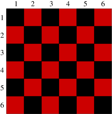
this choice can be illustrated by reference to a checkerboard of red
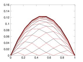
and black squares representing the positions of the nodes. Fig.&nbsp;<a href="chap6.xml#fig:redblack">6.1</a> illustrates the approach. The algorithm is to
update first the red, then the black squares. The Red-Black updating
order separates the update into two<a 
id="red-black_order62361"></a>
half-updates.<a href="footnote.xml#tthFtNtADG" id="tthFrefADG"><math xmlns="http://www.w3.org/1998/Math/MathML">
<mrow>
<msup><mrow></mrow><mrow><mn>36</mn></mrow>
</msup>
</mrow></math></a>

<div class="p"><!----></div>
<a id="tth_fIg6.1">
</a>   <img src="figures/redblackiter.png" alt="figures/redblackiter.png" /><a id="redblackiter">
</a>(a)<img src="figures/checkers.png" alt="figures/checkers.png" /><a id="checkers">
</a>(b)&nbsp;  
<div style="text-align:center">Figure 6.1: (a) One dimensional Gauss Seidel odd-even iteration produces
    successive solutions for each half-step that form a web that
    progresses upwards toward the solution. (b) In two dimensions the
    alternate squares to be updated are all the red (lighter shaded), then all the black.</div>
  <a id="fig:redblack">
</a>

<div class="p"><!----></div>
Consider a Fourier<a 
id="Fourier_representation62362"></a> mode<a href="footnote.xml#tthFtNtADH" id="tthFrefADH"><math xmlns="http://www.w3.org/1998/Math/MathML">
<mrow>
<msup><mrow></mrow><mrow><mn>37</mn></mrow>
</msup>
</mrow></math></a> of wave number <math xmlns="http://www.w3.org/1998/Math/MathML">
<mrow>
<msub><mrow><mi>k</mi></mrow><mrow><mi>x</mi></mrow>
</msub>
<mo>=</mo><mi>p</mi><mi mathvariant="italic">&pi;</mi><mo stretchy="false">/</mo><mi>L</mi></mrow></math>, where <math xmlns="http://www.w3.org/1998/Math/MathML">
<mrow><mi>p</mi></mrow></math> is the
integer mode number and <math xmlns="http://www.w3.org/1998/Math/MathML">
<mrow><mi>L</mi></mrow></math> is the length of the domain
(one-dimensional for simplicity) at whose ends Dirichlet boundary
conditions are assumed. Its half-update through eq.&nbsp;(<a href="chap6.xml#Jacobi">6.6</a>) (ignoring the source term), gives rise to an
amplification factor<a 
id="amplification_factor_Gauss-Seidel62363"></a>
<a id="GSamplific">
</a><br />
<table width="100%"><tr><td align="center">
    <math xmlns="http://www.w3.org/1998/Math/MathML">
    <mstyle displaystyle="true"><mrow><mi>A</mi><mo>=</mo>
<msubsup><mrow><mi mathvariant="italic">&psi;</mi></mrow><mrow><mi>j</mi> </mrow>
<mrow><mo stretchy="false">(</mo><mi>n</mi><mo>+</mo><mn>1</mn><mo stretchy="false">)</mo></mrow></msubsup>
<mo stretchy="false">/</mo>
<msubsup><mrow><mi mathvariant="italic">&psi;</mi></mrow><mrow><mi>j</mi> </mrow>
<mrow><mo stretchy="false">(</mo><mi>n</mi><mo stretchy="false">)</mo></mrow></msubsup>
<mo>=</mo>
<mfrac><mrow><mn>1</mn></mrow>
<mrow><mn>2</mn></mrow>
</mfrac>
<mo stretchy="false">(</mo>
<msup><mrow><mi fontstyle="normal">e</mi></mrow><mrow><mi mathvariant="italic">ip</mi><mi mathvariant="italic">&pi;</mi><mi mathvariant="italic">&Delta;</mi><mi>x</mi><mo stretchy="false">/</mo><mi>L</mi></mrow>
</msup>
<mo>+</mo>
<msup><mrow><mi fontstyle="normal">e</mi></mrow><mrow><mo>-</mo><mi mathvariant="italic">ip</mi><mi mathvariant="italic">&pi;</mi>
<msub><mrow><mi mathvariant="italic">&Delta;</mi></mrow><mrow><mi>x</mi></mrow>
</msub>
<mo stretchy="false">/</mo><mi>L</mi></mrow>
</msup>
<mo stretchy="false">)</mo><mo>=</mo><mi>cos</mi><mo stretchy="false">(</mo><mi>p</mi><mi mathvariant="italic">&pi;</mi><mi mathvariant="italic">&Delta;</mi><mi>x</mi><mo stretchy="false">/</mo><mi>L</mi><mo stretchy="false">)</mo></mrow>
    </mstyle></math></td><td width="1">
    <math xmlns="http://www.w3.org/1998/Math/MathML">
    <mstyle displaystyle="true"><mrow><mo stretchy="false">(</mo><mn>6</mn><mo>.</mo><mn>8</mn><mo stretchy="false">)</mo></mrow>
    </mstyle></math>
</td></tr></table>


The convergence process consists of the decay of the error in each mode of the
system, by which <math xmlns="http://www.w3.org/1998/Math/MathML">
<mrow><mi mathvariant="italic">&psi;</mi></mrow></math> is still different from
the steady solution. Each mode is repetitively multiplied by <math xmlns="http://www.w3.org/1998/Math/MathML">
<mrow><mi>A</mi></mrow></math> at
each half-step.  So after <math xmlns="http://www.w3.org/1998/Math/MathML">
<mrow><mi>m</mi></mrow></math> full-steps (<math xmlns="http://www.w3.org/1998/Math/MathML">
<mrow><mn>2</mn><mi>m</mi></mrow></math> half-steps) the mode
has decayed by a factor <math xmlns="http://www.w3.org/1998/Math/MathML">
<mrow>
<msup><mrow><mi>A</mi></mrow><mrow><mn>2</mn><mi>m</mi></mrow>
</msup>
</mrow></math>. After some time, the biggest error
is going to be caused by the slowest-decaying mode. That is the mode
whose amplitude factor is closest to 1. Since <math xmlns="http://www.w3.org/1998/Math/MathML">
<mrow><mi>A</mi><mo>=</mo><mi>cos</mi><mo stretchy="false">(</mo><mi>p</mi><mi mathvariant="italic">&pi;</mi><mi mathvariant="italic">&Delta;</mi><mi>x</mi><mo stretchy="false">/</mo><mi>L</mi><mo stretchy="false">)</mo></mrow></math>, the mode with <math xmlns="http://www.w3.org/1998/Math/MathML">
<mrow><mi>A</mi></mrow></math> closest to 1 is the mode with the smallest
wave number namely <math xmlns="http://www.w3.org/1998/Math/MathML">
<mrow><mi>p</mi><mo>=</mo><mn>1</mn></mrow></math>. If the number of spatial mesh nodes,
<math xmlns="http://www.w3.org/1998/Math/MathML">
<mrow>
<msub><mrow><mi>N</mi></mrow><mrow><mi>j</mi></mrow>
</msub>
<mo>=</mo><mi>L</mi><mo stretchy="false">/</mo><mi mathvariant="italic">&Delta;</mi><mi>x</mi></mrow></math> is large, then we can Taylor expand the cosine (for
<math xmlns="http://www.w3.org/1998/Math/MathML">
<mrow><mi>p</mi><mo>=</mo><mn>1</mn></mrow></math>)
<a id="GSapprox">
</a><br />
<table width="100%"><tr><td align="center">
    <math xmlns="http://www.w3.org/1998/Math/MathML">
    <mstyle displaystyle="true"><mrow><mi>A</mi><mo>&ap;</mo><mn>1</mn><mo>-</mo>
<mfrac><mrow><mn>1</mn></mrow>
<mrow><mn>2</mn></mrow>
</mfrac>

<msup><mrow><mo>(</mo>
<mfrac><mrow><mi mathvariant="italic">&pi;</mi><mi mathvariant="italic">&Delta;</mi><mi>x</mi></mrow>
<mrow><mi>L</mi></mrow>
</mfrac>
<mo>)</mo></mrow><mrow><mn>2</mn></mrow>
</msup>
<mo>=</mo><mn>1</mn><mo>-</mo>
<mfrac><mrow><mn>1</mn></mrow>
<mrow><mn>2</mn></mrow>
</mfrac>

<msup><mrow><mo>(</mo>
<mfrac><mrow><mi mathvariant="italic">&pi;</mi></mrow>
<mrow>
<msub><mrow><mi>N</mi></mrow><mrow><mi>j</mi></mrow>
</msub>
</mrow>
</mfrac>
<mo>)</mo></mrow><mrow><mn>2</mn></mrow>
</msup>
<mo>.</mo></mrow>
    </mstyle></math></td><td width="1">
    <math xmlns="http://www.w3.org/1998/Math/MathML">
    <mstyle displaystyle="true"><mrow><mo stretchy="false">(</mo><mn>6</mn><mo>.</mo><mn>9</mn><mo stretchy="false">)</mo></mrow>
    </mstyle></math>
</td></tr></table>


To reduce the amplitude of the mode by a factor <math xmlns="http://www.w3.org/1998/Math/MathML">
<mrow><mn>1</mn><mo stretchy="false">/</mo><mi>F</mi></mrow></math> takes a
number of steps <math xmlns="http://www.w3.org/1998/Math/MathML">
<mrow><mi>m</mi></mrow></math> such that <math xmlns="http://www.w3.org/1998/Math/MathML">
<mrow>
<msup><mrow><mi>A</mi></mrow><mrow><mn>2</mn><mi>m</mi></mrow>
</msup>
<mo>=</mo><mn>1</mn><mo stretchy="false">/</mo><mi>F</mi></mrow></math>, or, taking the logarithm
and using the expansion <math xmlns="http://www.w3.org/1998/Math/MathML">
<mrow><mi>ln</mi><mo stretchy="false">(</mo><mn>1</mn><mo>+</mo><mi>x</mi><mo stretchy="false">)</mo><mo>&ap;</mo><mi>x</mi></mrow></math>, so <math xmlns="http://www.w3.org/1998/Math/MathML">
<mrow><mi>ln</mi><mi>A</mi><mo>&ap;</mo><mo>-</mo>
<msup><mrow><mi mathvariant="italic">&pi;</mi></mrow><mrow><mn>2</mn></mrow>
</msup>
<mo stretchy="false">/</mo><mn>2</mn>
<msubsup><mrow><mi>N</mi></mrow><mrow><mi>j</mi> </mrow>
<mrow><mn>2</mn></mrow></msubsup>
</mrow></math>,
<a id="stepsreq">
</a><br />
<table width="100%"><tr><td align="center">
    <math xmlns="http://www.w3.org/1998/Math/MathML">
    <mstyle displaystyle="true"><mrow><mi>m</mi><mo>=</mo>
<mfrac><mrow><mn>1</mn></mrow>
<mrow><mn>2</mn></mrow>
</mfrac>
<mi>ln</mi><mo stretchy="false">(</mo><mn>1</mn><mo stretchy="false">/</mo><mi>F</mi><mo stretchy="false">)</mo><mo stretchy="false">/</mo><mi>ln</mi><mi>A</mi><mo>&ap;</mo><mi>ln</mi><mi>F</mi>
<msup><mrow><mo>(</mo>
<mfrac><mrow>
<msub><mrow><mi>N</mi></mrow><mrow><mi>j</mi></mrow>
</msub>
</mrow>
<mrow><mi mathvariant="italic">&pi;</mi></mrow>
</mfrac>
<mo>)</mo></mrow><mrow><mn>2</mn></mrow>
</msup>
<mo>.</mo></mrow>
    </mstyle></math></td><td width="1">
    <math xmlns="http://www.w3.org/1998/Math/MathML">
    <mstyle displaystyle="true"><mrow><mo stretchy="false">(</mo><mn>6</mn><mo>.</mo><mn>10</mn><mo stretchy="false">)</mo></mrow>
    </mstyle></math>
</td></tr></table>


This equation shows that to converge by a specified factor, requires a
number of steps proportional to <math xmlns="http://www.w3.org/1998/Math/MathML">
<mrow>
<msubsup><mrow><mi>N</mi></mrow><mrow><mi>j</mi> </mrow>
<mrow><mn>2</mn></mrow></msubsup>
</mrow></math>. That is a lot 
of<a 
id="convergence_Gauss-Seidel62364"></a>
iterations. Incidentally, the Jacobi iteration obviously leads to the
same amplification factor <math xmlns="http://www.w3.org/1998/Math/MathML">
<mrow><mi>A</mi></mrow></math>. The difference is that it is the factor
for a full step, rather than a half step. Therefore Gauss-Seidel
iteration converges only a factor of two faster than Jacobi iteration.
On the plus side, for multiple dimensions, things don't get
significantly worse. A square two-dimensional domain with <math xmlns="http://www.w3.org/1998/Math/MathML">
<mrow><mi mathvariant="italic">&Delta;</mi><mi>x</mi><mo>=</mo><mi mathvariant="italic">&Delta;</mi><mi>y</mi></mrow></math> has the same <math xmlns="http://www.w3.org/1998/Math/MathML">
<mrow><mi>A</mi></mrow></math>, so it takes the same number of iterations.

<div class="p"><!----></div>
 <a id="tth_sEc6.3"></a><h2>
6.3&nbsp;&nbsp;Successive Over-Relaxation</h2>

<div class="p"><!----></div>
<a 
id="successive_over-relaxation63365"></a><a 
id="SOR63366"></a><a 
id="over-relaxation63367"></a>The Gauss-Seidel method is a "successive" method where values are
updated in succession, and the
updated values are immediately used. It turns out that one can greatly
improve the convergence rate by the simple expedient of
over-correcting the error at each step. This is called
"over-relaxation" and when applied to the Gauss-Seidel method is
therefore called "Successive Over-Relaxation" or SOR. By analogy
with eq.&nbsp;(<a href="chap6.xml#Jacobi2">6.7</a>) it can be written
<a id="SORgen">
</a><br />
<table width="100%"><tr><td align="center">
    <math xmlns="http://www.w3.org/1998/Math/MathML">
    <mstyle displaystyle="true"><mrow>
<msubsup><mrow><mi mathvariant="italic">&psi;</mi></mrow><mrow><mi>j</mi> </mrow>
<mrow><mo stretchy="false">(</mo><mi>n</mi><mo>+</mo><mn>1</mn><mo stretchy="false">)</mo></mrow></msubsup>
<mo>-</mo>
<msubsup><mrow><mi mathvariant="italic">&psi;</mi></mrow><mrow><mi>j</mi> </mrow>
<mrow><mo stretchy="false">(</mo><mi>n</mi><mo stretchy="false">)</mo></mrow></msubsup>
<mo>=</mo><mi mathvariant="italic">&omega;</mi><mrow><mo>[</mo><mi>&emsp;</mi><mrow><mo>(</mo>
<munder><mo>&sum;</mo><mrow><mi>q</mi></mrow>
</munder>

<msub><mrow><mi>a</mi></mrow><mrow><mi>q</mi></mrow>
</msub>

<msubsup><mrow><mi mathvariant="italic">&psi;</mi></mrow><mrow><mi>q</mi> </mrow>
<mrow><mo stretchy="false">(</mo><mi>r</mi><mo stretchy="false">)</mo></mrow></msubsup>
<mrow><mo> </mo><mo>/</mo></mrow>
<munder><mo>&sum;</mo><mrow><mi>q</mi></mrow>
</munder>

<msub><mrow><mi>a</mi></mrow><mrow><mi>q</mi></mrow>
</msub>
<mo>)</mo></mrow><mo>-</mo>
<msubsup><mrow><mi mathvariant="italic">&psi;</mi></mrow><mrow><mi>j</mi> </mrow>
<mrow><mo stretchy="false">(</mo><mi>n</mi><mo stretchy="false">)</mo></mrow></msubsup>
<mo>+</mo>
<mfrac><mrow>
<msubsup><mrow><mi>s</mi></mrow><mrow><mi>j</mi> </mrow>
<mrow><mo stretchy="false">(</mo><mi>n</mi><mo stretchy="false">)</mo></mrow></msubsup>
<mi mathvariant="italic">&Delta;</mi><mi>t</mi></mrow>
<mrow>
<munder><mo>&sum;</mo><mrow><mi>q</mi></mrow>
</munder>

<msub><mrow><mi>a</mi></mrow><mrow><mi>q</mi></mrow>
</msub>
</mrow>
</mfrac>
<mo>]</mo></mrow><mo>,</mo></mrow>
    </mstyle></math></td><td width="1">
    <math xmlns="http://www.w3.org/1998/Math/MathML">
    <mstyle displaystyle="true"><mrow><mo stretchy="false">(</mo><mn>6</mn><mo>.</mo><mn>11</mn><mo stretchy="false">)</mo></mrow>
    </mstyle></math>
</td></tr></table>


where <math xmlns="http://www.w3.org/1998/Math/MathML">
<mrow><mi>r</mi><mo>=</mo><mi>n</mi></mrow></math> for <math xmlns="http://www.w3.org/1998/Math/MathML">
<mrow><mi>q</mi></mrow></math> corresponding to odd centered stencils, and
<math xmlns="http://www.w3.org/1998/Math/MathML">
<mrow><mi>r</mi><mo>=</mo><mi>n</mi><mo>+</mo><mn>1</mn></mrow></math> for <math xmlns="http://www.w3.org/1998/Math/MathML">
<mrow><mi>q</mi></mrow></math> corresponding to even.  The parameter <math xmlns="http://www.w3.org/1998/Math/MathML">
<mrow><mi mathvariant="italic">&omega;</mi><mo>&gt;</mo><mn>1</mn></mrow></math> is
the over-relaxation parameter. Strictly speaking, if <math xmlns="http://www.w3.org/1998/Math/MathML">
<mrow><mi mathvariant="italic">&omega;</mi><mo>&lt;</mo><mn>1</mn></mrow></math> one
should speak of under-relaxation. The particular case <math xmlns="http://www.w3.org/1998/Math/MathML">
<mrow><mi mathvariant="italic">&omega;</mi><mo>=</mo><mn>1</mn></mrow></math> is
the original Gauss-Seidel scheme.

<div class="p"><!----></div>
It turns out that SOR<a 
id="SOR_stability63368"></a> is stable for <math xmlns="http://www.w3.org/1998/Math/MathML">
<mrow><mn>0</mn><mo>&lt;</mo><mi mathvariant="italic">&omega;</mi><mo>&lt;</mo><mn>2</mn></mrow></math>.  It is intuitively
reasonable to guess that SOR converges faster for <math xmlns="http://www.w3.org/1998/Math/MathML">
<mrow><mi mathvariant="italic">&omega;</mi><mo>&gt;</mo><mn>1</mn></mrow></math>, than for
<math xmlns="http://www.w3.org/1998/Math/MathML">
<mrow><mi mathvariant="italic">&omega;</mi><mo>=</mo><mn>1</mn></mrow></math>.  It is not at all straightforward to show how much faster
it converges.<a href="footnote.xml#tthFtNtADI" id="tthFrefADI"><math xmlns="http://www.w3.org/1998/Math/MathML">
<mrow>
<msup><mrow></mrow><mrow><mn>38</mn></mrow>
</msup>
</mrow></math></a>  Therefore we will simply
summarize the facts without proving them.

<ul>
<li> There is an optimal<a 
id="SOR_optimal63369"></a> value of <math xmlns="http://www.w3.org/1998/Math/MathML">
<mrow><mi mathvariant="italic">&omega;</mi></mrow></math> somewhere between 1
and 2, where SOR converges fastest.
<div class="p"><!----></div>
</li>

<li> If <math xmlns="http://www.w3.org/1998/Math/MathML">
<mrow>
<msub><mrow><mi>A</mi></mrow><mrow><mi>J</mi></mrow>
</msub>
</mrow></math> is the amplification factor for the corresponding
  Jacobi iteration [<math xmlns="http://www.w3.org/1998/Math/MathML">
<mrow><mi>cos</mi><mo stretchy="false">(</mo><mi mathvariant="italic">&pi;</mi><mi mathvariant="italic">&Delta;</mi><mi>x</mi><mo stretchy="false">/</mo><mi>L</mi><mo stretchy="false">)</mo></mrow></math> for a uniform problem] then
  the optimal value is <math xmlns="http://www.w3.org/1998/Math/MathML">
<mrow><mi mathvariant="italic">&omega;</mi><mo>=</mo>
<msub><mrow><mi mathvariant="italic">&omega;</mi></mrow><mrow><mi>b</mi></mrow>
</msub>
<mo>=</mo><mn>2</mn><mo stretchy="false">/</mo><mo stretchy="false">(</mo><mn>1</mn><mo>+</mo><msqrt><mrow><mn>1</mn><mo>-</mo>
<msubsup><mrow><mi>A</mi></mrow><mrow><mi>J</mi> </mrow>
<mrow><mn>2</mn></mrow></msubsup>
</mrow></msqrt><mo stretchy="false">)</mo></mrow></math>.
<div class="p"><!----></div>
</li>

<li> For this optimal <math xmlns="http://www.w3.org/1998/Math/MathML">
<mrow><mi mathvariant="italic">&omega;</mi></mrow></math> the amplification factor for the SOR
  is <math xmlns="http://www.w3.org/1998/Math/MathML">
<mrow>
<msub><mrow><mi>A</mi></mrow><mrow><mi mathvariant="italic">SOR</mi></mrow>
</msub>
<mo>=</mo>
<msub><mrow><mi mathvariant="italic">&omega;</mi></mrow><mrow><mi>b</mi></mrow>
</msub>
<mo>-</mo><mn>1</mn><mo>=</mo><mo stretchy="false">(</mo>
<msub><mrow><mi>A</mi></mrow><mrow><mi>J</mi></mrow>
</msub>

<msub><mrow><mi mathvariant="italic">&omega;</mi></mrow><mrow><mi>b</mi></mrow>
</msub>
<mo stretchy="false">/</mo><mn>2</mn>
<msup><mrow><mo stretchy="false">)</mo></mrow><mrow><mn>2</mn></mrow>
</msup>
</mrow></math>.
For the uniform case and large <math xmlns="http://www.w3.org/1998/Math/MathML">
<mrow>
<msub><mrow><mi>N</mi></mrow><mrow><mi>j</mi></mrow>
</msub>
</mrow></math>, these imply
<a id="SORopt">
</a><br />
<table width="100%"><tr><td align="center">
    <math xmlns="http://www.w3.org/1998/Math/MathML">
    <mstyle displaystyle="true"><mrow>
<msub><mrow><mi mathvariant="italic">&omega;</mi></mrow><mrow><mi>b</mi></mrow>
</msub>
<mo>&ap;</mo>
<mfrac><mrow><mn>2</mn></mrow>
<mrow><mn>1</mn><mo>+</mo><mi mathvariant="italic">&pi;</mi><mo stretchy="false">/</mo>
<msub><mrow><mi>N</mi></mrow><mrow><mi>j</mi></mrow>
</msub>
</mrow>
</mfrac>
<mo>,</mo><mi>&emsp;&emsp;&emsp;&emsp;&emsp;&emsp;</mi>
<mtext>and</mtext>
<mi>&emsp;&emsp;&emsp;</mi>
<msub><mrow><mi>A</mi></mrow><mrow><mi mathvariant="italic">SOR</mi></mrow>
</msub>
<mo>&ap;</mo><mn>1</mn><mo>-</mo>
<mfrac><mrow><mn>2</mn><mi mathvariant="italic">&pi;</mi></mrow>
<mrow>
<msub><mrow><mi>N</mi></mrow><mrow><mi>j</mi></mrow>
</msub>
</mrow>
</mfrac>
<mo>.</mo></mrow>
    </mstyle></math></td><td width="1">
    <math xmlns="http://www.w3.org/1998/Math/MathML">
    <mstyle displaystyle="true"><mrow><mo stretchy="false">(</mo><mn>6</mn><mo>.</mo><mn>12</mn><mo stretchy="false">)</mo></mrow>
    </mstyle></math>
</td></tr></table>


<div class="p"><!----></div>
</li>
</ul>
These facts show that near the optimal relaxation parameter the number
of steps needed to converge by a factor <math xmlns="http://www.w3.org/1998/Math/MathML">
<mrow><mi>F</mi></mrow></math> is approximately <math xmlns="http://www.w3.org/1998/Math/MathML">
<mrow>
<msub><mrow><mi>N</mi></mrow><mrow><mi>j</mi></mrow>
</msub>
<mi>ln</mi><mi>F</mi><mo stretchy="false">/</mo><mn>2</mn><mi mathvariant="italic">&pi;</mi></mrow></math>
(not <math xmlns="http://www.w3.org/1998/Math/MathML">
<mrow>
<msubsup><mrow><mi>N</mi></mrow><mrow><mi>j</mi> </mrow>
<mrow><mn>2</mn></mrow></msubsup>
<mi>ln</mi><mi>F</mi><mo stretchy="false">/</mo>
<msup><mrow><mi mathvariant="italic">&pi;</mi></mrow><mrow><mn>2</mn></mrow>
</msup>
</mrow></math> as with Gauss-Seidel)<a 
id="SOR_convergence63370"></a>. That is a very big
benefit. However, obtaining that benefit requires one to estimate
<math xmlns="http://www.w3.org/1998/Math/MathML">
<mrow>
<msub><mrow><mi mathvariant="italic">&omega;</mi></mrow><mrow><mi>b</mi></mrow>
</msub>
</mrow></math> accurately, and for more complicated problems doing that
becomes hard. Choosing <math xmlns="http://www.w3.org/1998/Math/MathML">
<mrow><mi mathvariant="italic">&omega;</mi></mrow></math> well is probably the main challenge
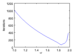
for SOR. Fig.&nbsp;<a href="chap6.xml#poisconverge">6.2</a> shows an illustrative example.

<div class="p"><!----></div>
<a id="tth_fIg6.2">
</a>   <img src="figures/convergence.png" alt="figures/convergence.png" /><a id="convergence">
</a>
  
<div style="text-align:center">Figure 6.2: Number of iterations required to converge a SOR solution of
    Poisson's equation with uniform source on a mesh of length
    <math xmlns="http://www.w3.org/1998/Math/MathML">
<mrow>
<msub><mrow><mi>N</mi></mrow><mrow><mi>j</mi></mrow>
</msub>
<mo>=</mo><mn>32</mn></mrow></math>. It is declared converged when the maximum <math xmlns="http://www.w3.org/1998/Math/MathML">
<mrow><mi mathvariant="italic">&psi;</mi></mrow></math>-change
    in a step is less than <math xmlns="http://www.w3.org/1998/Math/MathML">
<mrow>
<msup><mrow><mn>10</mn></mrow><mrow><mo>-</mo><mn>6</mn></mrow>
</msup>

<msub><mrow><mi mathvariant="italic">&psi;</mi></mrow><mrow><mi fontstyle="normal">max</mi></mrow>
</msub>
</mrow></math>. The minimum
    number of iterations is found to be 63 at <math xmlns="http://www.w3.org/1998/Math/MathML">
<mrow><mi mathvariant="italic">&omega;</mi><mo>=</mo><mn>1</mn><mo>.</mo><mn>85</mn></mrow></math>. This
    should be compared with theoretical values of
    <math xmlns="http://www.w3.org/1998/Math/MathML">
<mrow><mi>ln</mi><mo stretchy="false">(</mo>
<msup><mrow><mn>10</mn></mrow><mrow><mn>6</mn></mrow>
</msup>
<mo stretchy="false">)</mo><mo stretchy="false">(</mo>
<msub><mrow><mi>N</mi></mrow><mrow><mi>j</mi></mrow>
</msub>
<mo stretchy="false">/</mo><mn>2</mn><mi mathvariant="italic">&pi;</mi><mo stretchy="false">)</mo><mo>=</mo><mn>70</mn></mrow></math> at
    <math xmlns="http://www.w3.org/1998/Math/MathML">
<mrow><mi mathvariant="italic">&omega;</mi><mo>=</mo><mn>2</mn><mo stretchy="false">/</mo><mo stretchy="false">(</mo><mn>1</mn><mo>+</mo><mi mathvariant="italic">&pi;</mi><mo stretchy="false">/</mo>
<msub><mrow><mi>N</mi></mrow><mrow><mi>j</mi></mrow>
</msub>
<mo stretchy="false">)</mo><mo>=</mo><mn>1</mn><mo>.</mo><mn>821</mn></mrow></math>.<a id="poisconverge">
</a></div>

<div class="p"><!----></div>
There are other iterative matrix solution techniques, associated with
the name Krylov<a 
id="Krylov63371"></a>. Like the SOR solution technique, they
use just multiplication by the matrix, not inversion. That is a big
advantage for very sparse matrices arising in PDE solving. They go by
names like "Conjugate Gradient"<a 
id="conjugate_gradient63372"></a>, "Newton
Krylov"<a 
id="Newton-Krylov63373"></a> and "GMRES"<a 
id="GMRES63374"></a>. In some
situations they converge faster than SOR, and they don't require
careful adjustment of a relaxation parameter. However, they have their
own tuning problems associated with "preconditioning". These topics
are introduced very briefly in the final chapter.

<div class="p"><!----></div>
 <a id="tth_sEc6.4"></a><h2>
6.4&nbsp;&nbsp;Iteration and Nonlinear Equations</h2>

<div class="p"><!----></div>
<a 
id="iteration64375"></a><a 
id="nonlinear_equations64376"></a> A major advantage accrues
to iterative methods of solving elliptic problems. It is that we
only have to <em>multiply by</em> the difference matrix. Because that
difference matrix is extremely sparse<a 
id="sparse64377"></a>, we need never in
fact construct it in its entirety. We perform the matrix
multiplication more physically by performing the small number of
multiplications of adjacent stencil mesh values by coefficients. This
saves immense amounts of storage space (compared with constructing the
full matrix), and immense numbers of irrelevant multiplications by
zero. The cost we must pay for the benefit of not constructing and
inverting the matrix is that a substantial number of iterations is
necessary. Generally for sizable multidimensional problems that
iteration cost is far less than the savings.

<div class="p"><!----></div>
Another situation where iteration becomes essential is when the
differential equations are
<em>nonlinear</em><a 
id="nonlinear_iteration64378"></a>. In the screening of
electric fields by plasmas<a 
id="plasma64379"></a> or
electrolytes<a 
id="electric_screening64380"></a>, for example, the source of the
Poisson equation (the charge density) is a nonlinear function of the
potential, <math xmlns="http://www.w3.org/1998/Math/MathML">
<mrow><mi mathvariant="italic">&phi;</mi></mrow></math>, in this case an exponential leading to:
<a id="nonlinpois">
</a><br />
<table width="100%"><tr><td align="center">
    <math xmlns="http://www.w3.org/1998/Math/MathML">
    <mstyle displaystyle="true"><mrow>
<msup><mrow><mo>&nabla;</mo></mrow><mrow><mn>2</mn></mrow>
</msup>
<mi mathvariant="italic">&phi;</mi><mo>=</mo><mo>-</mo><mi>s</mi><mo>=</mo><mi>exp</mi><mo stretchy="false">(</mo><mi mathvariant="italic">&phi;</mi><mo stretchy="false">)</mo><mo>-</mo><mn>1</mn><mo>.</mo></mrow>
    </mstyle></math></td><td width="1">
    <math xmlns="http://www.w3.org/1998/Math/MathML">
    <mstyle displaystyle="true"><mrow><mo stretchy="false">(</mo><mn>6</mn><mo>.</mo><mn>13</mn><mo stretchy="false">)</mo></mrow>
    </mstyle></math>
</td></tr></table>


How do we solve such an elliptic equation? It cannot be solved by
matrix inversion because of the nonlinearity on the right hand side.
Even if we invert the difference matrix and construct eq.&nbsp;(<a href="chap6.xml#invertBsol">6.3</a>): <math xmlns="http://www.w3.org/1998/Math/MathML">
<mrow>\upphi<mo>=</mo><mo>-</mo>
<msup><mrow><mi mathvariant="bold">B</mi></mrow><mrow><mo>-</mo><mn>1</mn></mrow>
</msup>
<mi mathvariant="bold">s</mi></mrow></math>, because <math xmlns="http://www.w3.org/1998/Math/MathML">
<mrow><mi>s</mi></mrow></math>
is a nonlinear function of <math xmlns="http://www.w3.org/1998/Math/MathML">
<mrow><mi mathvariant="italic">&phi;</mi></mrow></math>, this expression does not constitute
a solution of the problem. 

<div class="p"><!----></div>
The generic answer to how to solve a nonlinear<a 
id="linearization64381"></a> problem is

<ol type="1">
<li> Linearize it about the current estimate of the solution.
<div class="p"><!----></div>
</li>

<li> Solve or advance the linear problem.
<div class="p"><!----></div>
</li>

<li> Repeat from 1, until converged on the nonlinear solution.
<div class="p"><!----></div>
</li>
</ol>
When one knows that iteration is required anyway, because the problem
is nonlinear, one has substantial incentive to use an iterative
method for the linearized part of the problem as well. Very often it
will cost no more effort to solve a nonlinear problem by iteration
than a linear problem.

<div class="p"><!----></div>
     <a id="tth_sEc6.4.1"></a><h3>
6.4.1&nbsp;&nbsp;Linearization</h3>

<div class="p"><!----></div>
<a 
id="linearization64382"></a>Suppose we have potential function <math xmlns="http://www.w3.org/1998/Math/MathML">
<mrow>
<msup><mrow><mi mathvariant="italic">&phi;</mi></mrow><mrow><mo stretchy="false">(</mo><mi>n</mi><mo stretchy="false">)</mo></mrow>
</msup>
</mrow></math>, at step <math xmlns="http://www.w3.org/1998/Math/MathML">
<mrow><mi>n</mi></mrow></math>, not yet
a solution of the steady elliptic equation. In the neighborhood of
that function, we can express the source via a Taylor
expansion<a 
id="Taylor_expansion64383"></a> (at
each point in the mesh):
<a id="nonlintaylor">
</a><br />
<table width="100%"><tr><td align="center">
    <math xmlns="http://www.w3.org/1998/Math/MathML">
    <mstyle displaystyle="true"><mrow><mi>s</mi><mo stretchy="false">(</mo><mi mathvariant="italic">&phi;</mi><mo stretchy="false">)</mo><mo>=</mo><mi>s</mi><mo stretchy="false">(</mo>
<msup><mrow><mi mathvariant="italic">&phi;</mi></mrow><mrow><mo stretchy="false">(</mo><mi>n</mi><mo stretchy="false">)</mo></mrow>
</msup>
<mo stretchy="false">)</mo><mo>+</mo>
<mfrac><mrow><mo>&part;</mo><mi>s</mi></mrow>
<mrow><mo>&part;</mo><mi mathvariant="italic">&phi;</mi></mrow>
</mfrac>

<mover><mrow><mi mathvariant="italic">&phi;</mi></mrow>
<mo>~</mo></mover>
<mo>+</mo>
<mfrac><mrow><mn>1</mn></mrow>
<mrow><mn>2</mn><mo>!</mo></mrow>
</mfrac>

<mfrac><mrow>
<msup><mrow><mo>&part;</mo></mrow><mrow><mn>2</mn></mrow>
</msup>
<mi>s</mi></mrow>
<mrow><mo>&part;</mo>
<msup><mrow><mi mathvariant="italic">&phi;</mi></mrow><mrow><mn>2</mn></mrow>
</msup>
</mrow>
</mfrac>

<msup><mrow>
<mover><mrow><mi mathvariant="italic">&phi;</mi></mrow>
<mo>~</mo></mover>
</mrow><mrow><mn>2</mn></mrow>
</msup>
<mo>&#x2026;</mo><mo>,</mo><mi>&emsp;&emsp;&emsp;&emsp;&emsp;&emsp;</mi>
<mtext>where</mtext>
<mi>&emsp;&emsp;&emsp;</mi>
<mover><mrow><mi mathvariant="italic">&phi;</mi></mrow>
<mo>~</mo></mover>
<mo>=</mo><mo stretchy="false">(</mo><mi mathvariant="italic">&phi;</mi><mo>-</mo>
<msup><mrow><mi mathvariant="italic">&phi;</mi></mrow><mrow><mo stretchy="false">(</mo><mi>n</mi><mo stretchy="false">)</mo></mrow>
</msup>
<mo stretchy="false">)</mo><mo>.</mo></mrow>
    </mstyle></math></td><td width="1">
    <math xmlns="http://www.w3.org/1998/Math/MathML">
    <mstyle displaystyle="true"><mrow><mo stretchy="false">(</mo><mn>6</mn><mo>.</mo><mn>14</mn><mo stretchy="false">)</mo></mrow>
    </mstyle></math>
</td></tr></table>


For values of <math xmlns="http://www.w3.org/1998/Math/MathML">
<mrow><mi mathvariant="italic">&phi;</mi></mrow></math> close enough to <math xmlns="http://www.w3.org/1998/Math/MathML">
<mrow>
<msup><mrow><mi mathvariant="italic">&phi;</mi></mrow><mrow><mo stretchy="false">(</mo><mi>n</mi><mo stretchy="false">)</mo></mrow>
</msup>
</mrow></math>, i.e. small enough
<math xmlns="http://www.w3.org/1998/Math/MathML">
<mrow>
<mover><mrow><mi mathvariant="italic">&phi;</mi></mrow>
<mo>~</mo></mover>
</mrow></math>, we can ignore all but the first two terms of this
expansion. For our exponential example, substituting for <math xmlns="http://www.w3.org/1998/Math/MathML">
<mrow><mi mathvariant="italic">&phi;</mi></mrow></math> and
rearranging the terms, we would then obtain the linearized equation
<a id="linshield">
</a><br />
<table width="100%"><tr><td align="center">
    <math xmlns="http://www.w3.org/1998/Math/MathML">
    <mstyle displaystyle="true"><mrow>
<msup><mrow><mo>&nabla;</mo></mrow><mrow><mn>2</mn></mrow>
</msup>

<mover><mrow><mi mathvariant="italic">&phi;</mi></mrow>
<mo>~</mo></mover>
<mo>-</mo><mi>exp</mi><mo stretchy="false">(</mo>
<msup><mrow><mi mathvariant="italic">&phi;</mi></mrow><mrow><mo stretchy="false">(</mo><mi>n</mi><mo stretchy="false">)</mo></mrow>
</msup>
<mo stretchy="false">)</mo>
<mover><mrow><mi mathvariant="italic">&phi;</mi></mrow>
<mo>~</mo></mover>
<mo>=</mo><mi>exp</mi><mo stretchy="false">(</mo>
<msup><mrow><mi mathvariant="italic">&phi;</mi></mrow><mrow><mo stretchy="false">(</mo><mi>n</mi><mo stretchy="false">)</mo></mrow>
</msup>
<mo stretchy="false">)</mo><mo>-</mo><mn>1</mn><mo>-</mo>
<msup><mrow><mo>&nabla;</mo></mrow><mrow><mn>2</mn></mrow>
</msup>

<msup><mrow><mi mathvariant="italic">&phi;</mi></mrow><mrow><mo stretchy="false">(</mo><mi>n</mi><mo stretchy="false">)</mo></mrow>
</msup>
<mo>.</mo></mrow>
    </mstyle></math></td><td width="1">
    <math xmlns="http://www.w3.org/1998/Math/MathML">
    <mstyle displaystyle="true"><mrow><mo stretchy="false">(</mo><mn>6</mn><mo>.</mo><mn>15</mn><mo stretchy="false">)</mo></mrow>
    </mstyle></math>
</td></tr></table>


The right hand side is the residual<a 
id="residual64384"></a> - the amount by which the
step-<math xmlns="http://www.w3.org/1998/Math/MathML">
<mrow><mi>n</mi></mrow></math> value fails to satisfy the differential equation.
More generally one obtains, from <math xmlns="http://www.w3.org/1998/Math/MathML">
<mrow>
<msup><mrow><mo>&nabla;</mo></mrow><mrow><mn>2</mn></mrow>
</msup>
<mi mathvariant="italic">&phi;</mi><mo>=</mo><mo>-</mo><mi>s</mi></mrow></math>, a linearized equation
<a id="lingen">
</a><br />
<table width="100%"><tr><td align="center">
    <math xmlns="http://www.w3.org/1998/Math/MathML">
    <mstyle displaystyle="true"><mrow>
<msup><mrow><mo>&nabla;</mo></mrow><mrow><mn>2</mn></mrow>
</msup>

<mover><mrow><mi mathvariant="italic">&phi;</mi></mrow>
<mo>~</mo></mover>
<mo>+</mo>
<msub><mrow><mo> </mo>
<mfrac><mrow><mo>&part;</mo><mi>s</mi></mrow>
<mrow><mo>&part;</mo><mi mathvariant="italic">&phi;</mi></mrow>
</mfrac>
<mo>|</mo></mrow><mrow>
<msup><mrow><mi mathvariant="italic">&phi;</mi></mrow><mrow><mo stretchy="false">(</mo><mi>n</mi><mo stretchy="false">)</mo></mrow>
</msup>
</mrow>
</msub>

<mover><mrow><mi mathvariant="italic">&phi;</mi></mrow>
<mo>~</mo></mover>
<mo>=</mo><mo>-</mo><mi>s</mi><mo stretchy="false">(</mo>
<msup><mrow><mi mathvariant="italic">&phi;</mi></mrow><mrow><mo stretchy="false">(</mo><mi>n</mi><mo stretchy="false">)</mo></mrow>
</msup>
<mo stretchy="false">)</mo><mo>-</mo>
<msup><mrow><mo>&nabla;</mo></mrow><mrow><mn>2</mn></mrow>
</msup>

<msup><mrow><mi mathvariant="italic">&phi;</mi></mrow><mrow><mo stretchy="false">(</mo><mi>n</mi><mo stretchy="false">)</mo></mrow>
</msup>
<mo>.</mo></mrow>
    </mstyle></math></td><td width="1">
    <math xmlns="http://www.w3.org/1998/Math/MathML">
    <mstyle displaystyle="true"><mrow><mo stretchy="false">(</mo><mn>6</mn><mo>.</mo><mn>16</mn><mo stretchy="false">)</mo></mrow>
    </mstyle></math>
</td></tr></table>


This equation can be solved to find <math xmlns="http://www.w3.org/1998/Math/MathML">
<mrow>
<mover><mrow><mi mathvariant="italic">&phi;</mi></mrow>
<mo>~</mo></mover>
</mrow></math> linearly. Of course
<math xmlns="http://www.w3.org/1998/Math/MathML">
<mrow>
<mover><mrow><mi mathvariant="italic">&phi;</mi></mrow>
<mo>~</mo></mover>
</mrow></math> is our linearized estimate of the amount by which the
real solution <math xmlns="http://www.w3.org/1998/Math/MathML">
<mrow><mi mathvariant="italic">&phi;</mi></mrow></math> is different from the starting value at the <math xmlns="http://www.w3.org/1998/Math/MathML">
<mrow><mi>n</mi></mrow></math>th
step: <math xmlns="http://www.w3.org/1998/Math/MathML">
<mrow>
<msup><mrow><mi mathvariant="italic">&phi;</mi></mrow><mrow><mo stretchy="false">(</mo><mi>n</mi><mo stretchy="false">)</mo></mrow>
</msup>
</mrow></math>. If we find the solution of the <em>linearized</em>
equation (<a href="chap6.xml#lingen">6.16</a>), then, since that equation is only
approximate, the new value <math xmlns="http://www.w3.org/1998/Math/MathML">
<mrow>
<msup><mrow><mi mathvariant="italic">&phi;</mi></mrow><mrow><mo stretchy="false">(</mo><mi>n</mi><mo>+</mo><mn>1</mn><mo stretchy="false">)</mo></mrow>
</msup>
<mo>&equiv;</mo>
<msup><mrow><mi mathvariant="italic">&phi;</mi></mrow><mrow><mo stretchy="false">(</mo><mi>n</mi><mo stretchy="false">)</mo></mrow>
</msup>
<mo>+</mo>
<mover><mrow><mi mathvariant="italic">&phi;</mi></mrow>
<mo>~</mo></mover>
</mrow></math> is only an
approximate solution of the original nonlinear equation. Presumably,
though, it is closer to the actual solution. So if we simply interate
the process then as <math xmlns="http://www.w3.org/1998/Math/MathML">
<mrow><mi>n</mi></mrow></math> increases we approach the full nonlinear
solution.  That is an iterative solution to the nonlinear problem
using linearization.

<div class="p"><!----></div>
     <a id="tth_sEc6.4.2"></a><h3>
6.4.2&nbsp;&nbsp;Combining linear and nonlinear iteration</h3>

<div class="p"><!----></div>
<a 
id="nonlinear_iteration64385"></a>The question then arises: what method should we use to solve the linear
problem to find <math xmlns="http://www.w3.org/1998/Math/MathML">
<mrow>
<mover><mrow><mi mathvariant="italic">&phi;</mi></mrow>
<mo>~</mo></mover>
</mrow></math>? It is natural to be guided by the
knowledge that even if we solved the linear problem exactly, that
would not give us an exact solution of the nonlinear
problem. Therefore it is <em>unnecessary</em> to solve the linearized
equation exactly. And in many cases it is in fact not even necessary
to get close to the exact solution of the linearized equation for each
interation of the nonlinear equation. What we then can do is to say,
we'll solve the linearized equation iteratively, but we'll use
<em>only one step</em> in our solution. In other words, <math xmlns="http://www.w3.org/1998/Math/MathML">
<mrow>
<msup><mrow><mi mathvariant="italic">&phi;</mi></mrow><mrow><mo stretchy="false">(</mo><mi>n</mi><mo>+</mo><mn>1</mn><mo stretchy="false">)</mo></mrow>
</msup>
</mrow></math>
is arrived at by doing a single advance of the linearized equation
iterative scheme (e.g.&nbsp;a SOR advance). Then we recalculate <math xmlns="http://www.w3.org/1998/Math/MathML">
<mrow><mi>s</mi></mrow></math> and
its derivative <math xmlns="http://www.w3.org/1998/Math/MathML">
<mrow><mo>&part;</mo><mi>s</mi><mo stretchy="false">/</mo><mo>&part;</mo><mi mathvariant="italic">&phi;</mi></mrow></math> for the new value of <math xmlns="http://www.w3.org/1998/Math/MathML">
<mrow><mi mathvariant="italic">&phi;</mi></mrow></math>,
and iterate. 

<div class="p"><!----></div>
Actually one might sometimes be able to dispense with the linear term
in the linearization, by retaining, in the Taylor expansion for <math xmlns="http://www.w3.org/1998/Math/MathML">
<mrow><mi>s</mi></mrow></math>,
only the first, constant term. That would amount to using
<math xmlns="http://www.w3.org/1998/Math/MathML">
<mrow>
<msup><mrow><mo>&nabla;</mo></mrow><mrow><mn>2</mn></mrow>
</msup>

<msup><mrow><mi mathvariant="italic">&phi;</mi></mrow><mrow><mo stretchy="false">(</mo><mi>n</mi><mo>+</mo><mn>1</mn><mo stretchy="false">)</mo></mrow>
</msup>
<mo>=</mo><mi>exp</mi>
<msup><mrow><mi mathvariant="italic">&phi;</mi></mrow><mrow><mo stretchy="false">(</mo><mi>n</mi><mo stretchy="false">)</mo></mrow>
</msup>
<mo>-</mo><mn>1</mn></mrow></math> as the equation to be solved
for each step of the nonlinear iteration. Whether that will work
depends upon the relative importance of the <math xmlns="http://www.w3.org/1998/Math/MathML">
<mrow>
<msup><mrow><mo>&nabla;</mo></mrow><mrow><mn>2</mn></mrow>
</msup>
<mi mathvariant="italic">&phi;</mi></mrow></math> term in the
equation. In places where <math xmlns="http://www.w3.org/1998/Math/MathML">
<mrow>
<msup><mrow><mo>&nabla;</mo></mrow><mrow><mn>2</mn></mrow>
</msup>
<mi mathvariant="italic">&phi;</mi></mrow></math> is small, the nonlinear
equation behaves like a transcendental equation for <math xmlns="http://www.w3.org/1998/Math/MathML">
<mrow><mi mathvariant="italic">&phi;</mi></mrow></math>: simply
<math xmlns="http://www.w3.org/1998/Math/MathML">
<mrow><mi>exp</mi><mi mathvariant="italic">&phi;</mi><mo>-</mo><mn>1</mn><mo>&ap;</mo><mn>0</mn></mrow></math>. In that case, solving eq.&nbsp;(<a href="chap6.xml#linshield">6.15</a>),
(without the <math xmlns="http://www.w3.org/1998/Math/MathML">
<mrow>
<msup><mrow><mo>&nabla;</mo></mrow><mrow><mn>2</mn></mrow>
</msup>
<mi mathvariant="italic">&phi;</mi></mrow></math> term) is equivalent to a single Newton
iteration<a 
id="Newton_method64386"></a> of a root-finding problem, which is a
sensible iteration to take. Without the linear term, though,
negligibly small advance towards the nonlinear solution will occur.

<div class="p"><!----></div>
It is hard to generalize about how fast the iteration is going to
converge on the solution of the nonlinear equation. It depends upon
the type of nonlinearity. But it is usually the case that if the
iterative advance is chosen reasonably, then the convergence to the
nonlinear solution takes no more iterations than approximately what it
would require to converge as accurately to a solution of the
linearized equations. In short, iterative solutions can readily
accommodate nonlinearity in the equations, and produce solutions with
comparable computational cost. 

<div class="p"><!----></div>

<h2>Worked Example: Optimal SOR relaxation</h2>

<div class="p"><!----></div>
<a 
id="SOR_optimal64387"></a><a 
id="SOR_convergence64388"></a>Consider the elliptic equation 
<a id="wk6eq1">
</a><br />
<table width="100%"><tr><td align="center">
    <math xmlns="http://www.w3.org/1998/Math/MathML">
    <mstyle displaystyle="true"><mrow>
<mfrac><mrow>
<msup><mrow><mo>&part;</mo></mrow><mrow><mn>2</mn></mrow>
</msup>
<mi mathvariant="italic">&phi;</mi></mrow>
<mrow><mo>&part;</mo>
<msup><mrow><mi>x</mi></mrow><mrow><mn>2</mn></mrow>
</msup>
</mrow>
</mfrac>
<mo>+</mo>
<mfrac><mrow>
<msup><mrow><mo>&part;</mo></mrow><mrow><mn>2</mn></mrow>
</msup>
<mi mathvariant="italic">&phi;</mi></mrow>
<mrow><mo>&part;</mo>
<msup><mrow><mi>y</mi></mrow><mrow><mn>2</mn></mrow>
</msup>
</mrow>
</mfrac>
<mo>=</mo><mi>s</mi><mo stretchy="false">(</mo><mi>x</mi><mo>,</mo><mi>y</mi><mo stretchy="false">)</mo></mrow>
    </mstyle></math></td><td width="1">
    <math xmlns="http://www.w3.org/1998/Math/MathML">
    <mstyle displaystyle="true"><mrow><mo stretchy="false">(</mo><mn>6</mn><mo>.</mo><mn>17</mn><mo stretchy="false">)</mo></mrow>
    </mstyle></math>
</td></tr></table>


expressed on a cartesian grid <math xmlns="http://www.w3.org/1998/Math/MathML">
<mrow><mi>x</mi><mo>=</mo><mi>j</mi><mi mathvariant="italic">&Delta;</mi><mi>x</mi></mrow></math>, <math xmlns="http://www.w3.org/1998/Math/MathML">
<mrow><mi>j</mi><mo>=</mo><mn>0</mn><mo>,</mo><mn>1</mn><mo>,</mo><mo>&#x2026;</mo><mo>,</mo>
<msub><mrow><mi>N</mi></mrow><mrow><mi>x</mi></mrow>
</msub>
</mrow></math>;
<math xmlns="http://www.w3.org/1998/Math/MathML">
<mrow><mi>y</mi><mo>=</mo><mi>k</mi><mi mathvariant="italic">&Delta;</mi><mi>y</mi></mrow></math>, <math xmlns="http://www.w3.org/1998/Math/MathML">
<mrow><mi>k</mi><mo>=</mo><mn>0</mn><mo>,</mo><mn>1</mn><mo>,</mo><mo>&#x2026;</mo><mo>,</mo>
<msub><mrow><mi>N</mi></mrow><mrow><mi>y</mi></mrow>
</msub>
</mrow></math>. And suppose the boundary conditions
at <math xmlns="http://www.w3.org/1998/Math/MathML">
<mrow><mi>x</mi><mo>=</mo><mn>0</mn></mrow></math> and <math xmlns="http://www.w3.org/1998/Math/MathML">
<mrow>
<msub><mrow><mi>N</mi></mrow><mrow><mi>x</mi></mrow>
</msub>
<mi mathvariant="italic">&Delta;</mi><mi>x</mi></mrow></math>, and <math xmlns="http://www.w3.org/1998/Math/MathML">
<mrow><mi>y</mi><mo>=</mo><mn>0</mn></mrow></math> and <math xmlns="http://www.w3.org/1998/Math/MathML">
<mrow>
<msub><mrow><mi>N</mi></mrow><mrow><mi>y</mi></mrow>
</msub>
<mi mathvariant="italic">&Delta;</mi><mi>y</mi></mrow></math> are
<math xmlns="http://www.w3.org/1998/Math/MathML">
<mrow><mi mathvariant="italic">&phi;</mi><mo>=</mo><mi>f</mi><mo stretchy="false">(</mo><mi>x</mi><mo>,</mo><mi>y</mi><mo stretchy="false">)</mo></mrow></math>. Find the optimum relaxation parameter <math xmlns="http://www.w3.org/1998/Math/MathML">
<mrow><mi mathvariant="italic">&omega;</mi></mrow></math> for an SOR
iterative solution of the system, and the resulting convergence rate.
<div class="p"><!----></div>
<br /><a 
id="linearization64389"></a>Suppose the final solution of the system is denoted <math xmlns="http://www.w3.org/1998/Math/MathML">
<mrow>
<msub><mrow><mi mathvariant="italic">&phi;</mi></mrow><mrow><mi>s</mi></mrow>
</msub>
</mrow></math>. We can
define a new dependent variable <math xmlns="http://www.w3.org/1998/Math/MathML">
<mrow><mi mathvariant="italic">&psi;</mi><mo>=</mo><mi mathvariant="italic">&phi;</mi><mo>-</mo>
<msub><mrow><mi mathvariant="italic">&phi;</mi></mrow><mrow><mi>s</mi></mrow>
</msub>
</mrow></math>, which is the error
between some approximation of the solution (<math xmlns="http://www.w3.org/1998/Math/MathML">
<mrow><mi mathvariant="italic">&phi;</mi></mrow></math>) and the actual
solution. Of course, while we are in the process of finding the
solution, we don't know how to derive <math xmlns="http://www.w3.org/1998/Math/MathML">
<mrow><mi mathvariant="italic">&psi;</mi></mrow></math> from <math xmlns="http://www.w3.org/1998/Math/MathML">
<mrow><mi mathvariant="italic">&phi;</mi></mrow></math>, because we
don't yet know what <math xmlns="http://www.w3.org/1998/Math/MathML">
<mrow>
<msub><mrow><mi mathvariant="italic">&phi;</mi></mrow><mrow><mi>s</mi></mrow>
</msub>
</mrow></math> is. That fact does not affect the
following arguments.  Substituting for <math xmlns="http://www.w3.org/1998/Math/MathML">
<mrow><mi mathvariant="italic">&phi;</mi><mo>=</mo><mi mathvariant="italic">&psi;</mi><mo>+</mo>
<msub><mrow><mi mathvariant="italic">&phi;</mi></mrow><mrow><mi>s</mi></mrow>
</msub>
</mrow></math> in the
differential equation and using the fact that <math xmlns="http://www.w3.org/1998/Math/MathML">
<mrow>
<msub><mrow><mi mathvariant="italic">&phi;</mi></mrow><mrow><mi>s</mi></mrow>
</msub>
</mrow></math> exactly
satisfies it and the boundary conditions, we immediately deduce that
<math xmlns="http://www.w3.org/1998/Math/MathML">
<mrow><mi mathvariant="italic">&psi;</mi></mrow></math> satisfies the homogeneous differential
equation<a 
id="homogeneous_equation64390"></a>
<a id="wk6eq2">
</a><br />
<table width="100%"><tr><td align="center">
    <math xmlns="http://www.w3.org/1998/Math/MathML">
    <mstyle displaystyle="true"><mrow>
<mfrac><mrow>
<msup><mrow><mo>&part;</mo></mrow><mrow><mn>2</mn></mrow>
</msup>
<mi mathvariant="italic">&psi;</mi></mrow>
<mrow><mo>&part;</mo>
<msup><mrow><mi>x</mi></mrow><mrow><mn>2</mn></mrow>
</msup>
</mrow>
</mfrac>
<mo>+</mo>
<mfrac><mrow>
<msup><mrow><mo>&part;</mo></mrow><mrow><mn>2</mn></mrow>
</msup>
<mi mathvariant="italic">&psi;</mi></mrow>
<mrow><mo>&part;</mo>
<msup><mrow><mi>y</mi></mrow><mrow><mn>2</mn></mrow>
</msup>
</mrow>
</mfrac>
<mo>=</mo><mn>0</mn><mo>,</mo></mrow>
    </mstyle></math></td><td width="1">
    <math xmlns="http://www.w3.org/1998/Math/MathML">
    <mstyle displaystyle="true"><mrow><mo stretchy="false">(</mo><mn>6</mn><mo>.</mo><mn>18</mn><mo stretchy="false">)</mo></mrow>
    </mstyle></math>
</td></tr></table>


together with homogeneous boundary conditions: <math xmlns="http://www.w3.org/1998/Math/MathML">
<mrow><mi mathvariant="italic">&psi;</mi><mo>=</mo><mn>0</mn></mrow></math> on the
boundary.  Of course the final solution for <math xmlns="http://www.w3.org/1998/Math/MathML">
<mrow><mi mathvariant="italic">&psi;</mi></mrow></math> is, as a
consequence, simply zero. But prior to arriving at that solution,
<math xmlns="http://www.w3.org/1998/Math/MathML">
<mrow><mi mathvariant="italic">&psi;</mi></mrow></math> is non-zero and any iteration scheme that we use to solve for
<math xmlns="http://www.w3.org/1998/Math/MathML">
<mrow><mi mathvariant="italic">&phi;</mi></mrow></math> is equivalent to an iteration scheme to solve for <math xmlns="http://www.w3.org/1998/Math/MathML">
<mrow><mi mathvariant="italic">&psi;</mi></mrow></math>. In
particular, the convergence rate of <math xmlns="http://www.w3.org/1998/Math/MathML">
<mrow><mi mathvariant="italic">&psi;</mi></mrow></math> to zero is just the
convergence rate of <math xmlns="http://www.w3.org/1998/Math/MathML">
<mrow><mi mathvariant="italic">&phi;</mi></mrow></math> to <math xmlns="http://www.w3.org/1998/Math/MathML">
<mrow>
<msub><mrow><mi mathvariant="italic">&phi;</mi></mrow><mrow><mi>s</mi></mrow>
</msub>
</mrow></math>. All stability and convergence
analysis can be done on the simpler homogeneous <math xmlns="http://www.w3.org/1998/Math/MathML">
<mrow><mi mathvariant="italic">&psi;</mi></mrow></math> system eq.&nbsp;(<a href="chap6.xml#wk6eq2">6.18</a>), and its results applied immediately to the <math xmlns="http://www.w3.org/1998/Math/MathML">
<mrow><mi mathvariant="italic">&phi;</mi></mrow></math>
system (<a href="chap6.xml#wk6eq1">6.17</a>).

<div class="p"><!----></div>
 The homogeneous Jacobi iteration<a 
id="Jacobi_method64391"></a>
(see eq.&nbsp;<a href="chap6.xml#Jacobi">6.6</a>) in two dimensions of different grid spacing is
<a id="Jacobi2d">
</a><br />
<table width="100%"><tr><td align="center">
    <math xmlns="http://www.w3.org/1998/Math/MathML">
    <mstyle displaystyle="true"><mrow>
<msubsup><mrow><mi mathvariant="italic">&psi;</mi></mrow><mrow><mi>j</mi><mo>,</mo><mi>k</mi> </mrow>
<mrow><mo stretchy="false">(</mo><mi>n</mi><mo>+</mo><mn>1</mn><mo stretchy="false">)</mo></mrow></msubsup>
<mo>-</mo>
<msubsup><mrow><mi mathvariant="italic">&psi;</mi></mrow><mrow><mi>j</mi><mo>,</mo><mi>k</mi> </mrow>
<mrow><mo stretchy="false">(</mo><mi>n</mi><mo stretchy="false">)</mo></mrow></msubsup>
<mo>=</mo>
<mfrac><mrow><mn>1</mn></mrow>
<mrow><mn>2</mn></mrow>
</mfrac>
<mrow><mo>(</mo>
<mfrac><mrow>
<msubsup><mrow><mi mathvariant="italic">&psi;</mi></mrow><mrow><mi>j</mi><mo>+</mo><mn>1</mn><mo>,</mo><mi>k</mi> </mrow>
<mrow><mo stretchy="false">(</mo><mi>n</mi><mo stretchy="false">)</mo></mrow></msubsup>
<mo>+</mo>
<msubsup><mrow><mi mathvariant="italic">&psi;</mi></mrow><mrow><mi>j</mi><mo>-</mo><mn>1</mn><mo>,</mo><mi>k</mi> </mrow>
<mrow><mo stretchy="false">(</mo><mi>n</mi><mo stretchy="false">)</mo></mrow></msubsup>
</mrow>
<mrow><mi mathvariant="italic">&Delta;</mi>
<msup><mrow><mi>x</mi></mrow><mrow><mn>2</mn></mrow>
</msup>
</mrow>
</mfrac>
<mo>+</mo>
<mfrac><mrow>
<msubsup><mrow><mi mathvariant="italic">&psi;</mi></mrow><mrow><mi>j</mi><mo>,</mo><mi>k</mi><mo>+</mo><mn>1</mn> </mrow>
<mrow><mo stretchy="false">(</mo><mi>n</mi><mo stretchy="false">)</mo></mrow></msubsup>
<mo>+</mo>
<msubsup><mrow><mi mathvariant="italic">&psi;</mi></mrow><mrow><mi>j</mi><mo>,</mo><mi>k</mi><mo>-</mo><mn>1</mn> </mrow>
<mrow><mo stretchy="false">(</mo><mi>n</mi><mo stretchy="false">)</mo></mrow></msubsup>
</mrow>
<mrow><mi mathvariant="italic">&Delta;</mi>
<msup><mrow><mi>y</mi></mrow><mrow><mn>2</mn></mrow>
</msup>
</mrow>
</mfrac>
<mo>)</mo></mrow>
<msup><mrow><mo>(</mo>
<mfrac><mrow><mn>1</mn></mrow>
<mrow><mi mathvariant="italic">&Delta;</mi>
<msup><mrow><mi>x</mi></mrow><mrow><mn>2</mn></mrow>
</msup>
</mrow>
</mfrac>
<mo>+</mo>
<mfrac><mrow><mn>1</mn></mrow>
<mrow><mi mathvariant="italic">&Delta;</mi>
<msup><mrow><mi>y</mi></mrow><mrow><mn>2</mn></mrow>
</msup>
</mrow>
</mfrac>
<mo>)</mo></mrow><mrow><mo>-</mo><mn>1</mn></mrow>
</msup>
<mo>-</mo>
<msubsup><mrow><mi mathvariant="italic">&psi;</mi></mrow><mrow><mi>j</mi><mo>,</mo><mi>k</mi> </mrow>
<mrow><mo stretchy="false">(</mo><mi>n</mi><mo stretchy="false">)</mo></mrow></msubsup>
<mo>.</mo></mrow>
    </mstyle></math></td><td width="1">
    <math xmlns="http://www.w3.org/1998/Math/MathML">
    <mstyle displaystyle="true"><mrow><mo stretchy="false">(</mo><mn>6</mn><mo>.</mo><mn>19</mn><mo stretchy="false">)</mo></mrow>
    </mstyle></math>
</td></tr></table>


Now we do a Von Neumann analysis of the 
homogeneous system<a 
id="Von_Neumann_stability64392"></a>, examining
the Fourier modes of the 2-Dimensional system. They are proportional
to <math xmlns="http://www.w3.org/1998/Math/MathML">
<mrow><mi>exp</mi><mi>i</mi><mo stretchy="false">(</mo>
<msub><mrow><mi>k</mi></mrow><mrow><mi>x</mi></mrow>
</msub>
<mi>x</mi><mo>+</mo>
<msub><mrow><mi>k</mi></mrow><mrow><mi>y</mi></mrow>
</msub>
<mi>y</mi><mo stretchy="false">)</mo><mo>=</mo><mi>exp</mi><mi>i</mi><mi mathvariant="italic">&pi;</mi><mo stretchy="false">(</mo><mi mathvariant="italic">pj</mi><mo stretchy="false">/</mo>
<msub><mrow><mi>N</mi></mrow><mrow><mi>x</mi></mrow>
</msub>
<mo>+</mo><mi mathvariant="italic">qk</mi><mo stretchy="false">/</mo>
<msub><mrow><mi>N</mi></mrow><mrow><mi>y</mi></mrow>
</msub>
<mo stretchy="false">)</mo></mrow></math>, where <math xmlns="http://www.w3.org/1998/Math/MathML">
<mrow><mi>p</mi></mrow></math> and <math xmlns="http://www.w3.org/1998/Math/MathML">
<mrow><mi>q</mi></mrow></math>
are integers that label the mode<a href="footnote.xml#tthFtNtADJ" id="tthFrefADJ"><math xmlns="http://www.w3.org/1998/Math/MathML">
<mrow>
<msup><mrow></mrow><mrow><mn>39</mn></mrow>
</msup>
</mrow></math></a>.
For the <math xmlns="http://www.w3.org/1998/Math/MathML">
<mrow><mi>p</mi><mo>,</mo><mi>q</mi></mrow></math> Fourier mode, <math xmlns="http://www.w3.org/1998/Math/MathML">
<mrow>
<msubsup><mrow><mi mathvariant="italic">&psi;</mi></mrow><mrow><mi>j</mi><mo>+</mo><mn>1</mn><mo>,</mo><mi>k</mi> </mrow>
<mrow><mo stretchy="false">(</mo><mi>n</mi><mo stretchy="false">)</mo></mrow></msubsup>
<mo>+</mo>
<msubsup><mrow><mi mathvariant="italic">&psi;</mi></mrow><mrow><mi>j</mi><mo>-</mo><mn>1</mn><mo>,</mo><mi>k</mi> </mrow>
<mrow><mo stretchy="false">(</mo><mi>n</mi><mo stretchy="false">)</mo></mrow></msubsup>
<mo>=</mo><mn>2</mn><mi>cos</mi><mo stretchy="false">(</mo><mi>p</mi><mi mathvariant="italic">&pi;</mi><mo stretchy="false">/</mo>
<msub><mrow><mi>N</mi></mrow><mrow><mi>x</mi></mrow>
</msub>
<mo stretchy="false">)</mo>
<msubsup><mrow><mi mathvariant="italic">&psi;</mi></mrow><mrow><mi>j</mi><mo>,</mo><mi>k</mi> </mrow>
<mrow><mo stretchy="false">(</mo><mi>n</mi><mo stretchy="false">)</mo></mrow></msubsup>
</mrow></math> and <math xmlns="http://www.w3.org/1998/Math/MathML">
<mrow>
<msubsup><mrow><mi mathvariant="italic">&psi;</mi></mrow><mrow><mi>j</mi><mo>,</mo><mi>k</mi><mo>+</mo><mn>1</mn> </mrow>
<mrow><mo stretchy="false">(</mo><mi>n</mi><mo stretchy="false">)</mo></mrow></msubsup>
<mo>+</mo>
<msubsup><mrow><mi mathvariant="italic">&psi;</mi></mrow><mrow><mi>j</mi><mo>,</mo><mi>k</mi><mo>-</mo><mn>1</mn> </mrow>
<mrow><mo stretchy="false">(</mo><mi>n</mi><mo stretchy="false">)</mo></mrow></msubsup>
<mo>=</mo><mn>2</mn><mi>cos</mi><mo stretchy="false">(</mo><mi>q</mi><mi mathvariant="italic">&pi;</mi><mo stretchy="false">/</mo>
<msub><mrow><mi>N</mi></mrow><mrow><mi>y</mi></mrow>
</msub>
<mo stretchy="false">)</mo>
<msubsup><mrow><mi mathvariant="italic">&psi;</mi></mrow><mrow><mi>j</mi><mo>,</mo><mi>k</mi> </mrow>
<mrow><mo stretchy="false">(</mo><mi>n</mi><mo stretchy="false">)</mo></mrow></msubsup>
</mrow></math>.
So, substituting, we get the two-dimensional version of eq.&nbsp;(<a href="chap6.xml#GSamplific">6.8</a>)
<a id="wk6eq5">
</a><br />
<table width="100%"><tr><td align="center">
    <math xmlns="http://www.w3.org/1998/Math/MathML">
    <mstyle displaystyle="true"><mrow>
<msub><mrow><mi>A</mi></mrow><mrow><mi>J</mi></mrow>
</msub>
<mo>&equiv;</mo>
<msubsup><mrow><mi mathvariant="italic">&psi;</mi></mrow><mrow><mi>j</mi><mo>,</mo><mi>k</mi> </mrow>
<mrow><mo stretchy="false">(</mo><mi>n</mi><mo>+</mo><mn>1</mn><mo stretchy="false">)</mo></mrow></msubsup>
<mo stretchy="false">/</mo>
<msubsup><mrow><mi mathvariant="italic">&psi;</mi></mrow><mrow><mi>j</mi><mo>,</mo><mi>k</mi> </mrow>
<mrow><mo stretchy="false">(</mo><mi>n</mi><mo stretchy="false">)</mo></mrow></msubsup>
<mo>=</mo><mrow><mo>(</mo>
<mfrac><mrow><mi>cos</mi><mo stretchy="false">(</mo><mi>p</mi><mi mathvariant="italic">&pi;</mi><mo stretchy="false">/</mo>
<msub><mrow><mi>N</mi></mrow><mrow><mi>x</mi></mrow>
</msub>
<mo stretchy="false">)</mo></mrow>
<mrow><mi mathvariant="italic">&Delta;</mi>
<msup><mrow><mi>x</mi></mrow><mrow><mn>2</mn></mrow>
</msup>
</mrow>
</mfrac>
<mo>+</mo>
<mfrac><mrow><mi>cos</mi><mo stretchy="false">(</mo><mi>q</mi><mi mathvariant="italic">&pi;</mi><mo stretchy="false">/</mo>
<msub><mrow><mi>N</mi></mrow><mrow><mi>y</mi></mrow>
</msub>
<mo stretchy="false">)</mo></mrow>
<mrow><mi mathvariant="italic">&Delta;</mi>
<msup><mrow><mi>y</mi></mrow><mrow><mn>2</mn></mrow>
</msup>
</mrow>
</mfrac>
<mo>)</mo></mrow>
<msup><mrow><mo>(</mo>
<mfrac><mrow><mn>1</mn></mrow>
<mrow><mi mathvariant="italic">&Delta;</mi>
<msup><mrow><mi>x</mi></mrow><mrow><mn>2</mn></mrow>
</msup>
</mrow>
</mfrac>
<mo>+</mo>
<mfrac><mrow><mn>1</mn></mrow>
<mrow><mi mathvariant="italic">&Delta;</mi>
<msup><mrow><mi>y</mi></mrow><mrow><mn>2</mn></mrow>
</msup>
</mrow>
</mfrac>
<mo>)</mo></mrow><mrow><mo>-</mo><mn>1</mn></mrow>
</msup>
<mo>.</mo></mrow>
    </mstyle></math></td><td width="1">
    <math xmlns="http://www.w3.org/1998/Math/MathML">
    <mstyle displaystyle="true"><mrow><mo stretchy="false">(</mo><mn>6</mn><mo>.</mo><mn>20</mn><mo stretchy="false">)</mo></mrow>
    </mstyle></math>
</td></tr></table>


The slowest-decaying mode is the longest wavelength mode: <math xmlns="http://www.w3.org/1998/Math/MathML">
<mrow><mi>p</mi><mo>=</mo><mn>1</mn></mrow></math>, <math xmlns="http://www.w3.org/1998/Math/MathML">
<mrow><mi>q</mi><mo>=</mo><mn>1</mn></mrow></math>.
For this mode, expanding <math xmlns="http://www.w3.org/1998/Math/MathML">
<mrow><mi>cos</mi><mi mathvariant="italic">&theta;</mi><mo>&ap;</mo><mn>1</mn><mo>-</mo>
<msup><mrow><mi mathvariant="italic">&theta;</mi></mrow><mrow><mn>2</mn></mrow>
</msup>
<mo stretchy="false">/</mo><mn>2</mn></mrow></math>, we get
<a id="wk6eq6">
</a><br />
<table width="100%"><tr><td align="center">
    <math xmlns="http://www.w3.org/1998/Math/MathML">
    <mstyle displaystyle="true"><mrow>
<mtable displaystyle="true" align="right" width="80%">
<mtr><mtd columnalign="right" columnspan="1"><mrow>
<msub><mrow><mi>A</mi></mrow><mrow><mi>J</mi></mrow>
</msub>
</mrow>
</mtd><mtd columnalign="left">
<mrow><mo>&ap;</mo></mrow>
</mtd><mtd columnalign="left">
<mrow><mn>1</mn><mo>-</mo><mrow><mo>(</mo>
<mfrac><mrow>
<msup><mrow><mi mathvariant="italic">&pi;</mi></mrow><mrow><mn>2</mn></mrow>
</msup>
</mrow>
<mrow><mn>2</mn>
<msubsup><mrow><mi>N</mi></mrow><mrow><mi>x</mi> </mrow>
<mrow><mn>2</mn></mrow></msubsup>
<mi mathvariant="italic">&Delta;</mi>
<msup><mrow><mi>x</mi></mrow><mrow><mn>2</mn></mrow>
</msup>
</mrow>
</mfrac>
<mo>+</mo>
<mfrac><mrow>
<msup><mrow><mi mathvariant="italic">&pi;</mi></mrow><mrow><mn>2</mn></mrow>
</msup>
</mrow>
<mrow><mn>2</mn>
<msubsup><mrow><mi>N</mi></mrow><mrow><mi>y</mi> </mrow>
<mrow><mn>2</mn></mrow></msubsup>
<mi mathvariant="italic">&Delta;</mi>
<msup><mrow><mi>y</mi></mrow><mrow><mn>2</mn></mrow>
</msup>
</mrow>
</mfrac>
<mo>)</mo></mrow>
<msup><mrow><mo>(</mo>
<mfrac><mrow><mn>1</mn></mrow>
<mrow><mi mathvariant="italic">&Delta;</mi>
<msup><mrow><mi>x</mi></mrow><mrow><mn>2</mn></mrow>
</msup>
</mrow>
</mfrac>
<mo>+</mo>
<mfrac><mrow><mn>1</mn></mrow>
<mrow><mi mathvariant="italic">&Delta;</mi>
<msup><mrow><mi>y</mi></mrow><mrow><mn>2</mn></mrow>
</msup>
</mrow>
</mfrac>
<mo>)</mo></mrow><mrow><mo>-</mo><mn>1</mn></mrow>
</msup>
</mrow>
</mtd></mtr>
<mtr><mtd columnalign="right" columnspan="1"><mrow></mrow>
</mtd><mtd columnalign="left">
<mrow><mo>=</mo></mrow>
</mtd><mtd columnalign="left">
<mrow><mn>1</mn><mo>-</mo>
<mfrac><mrow><mn>1</mn></mrow>
<mrow><mn>2</mn></mrow>
</mfrac>
<mrow><mo>[</mo>
<msup><mrow><mo>(</mo>
<mfrac><mrow><mi mathvariant="italic">&pi;</mi></mrow>
<mrow>
<msub><mrow><mi>N</mi></mrow><mrow><mi>x</mi></mrow>
</msub>
</mrow>
</mfrac>
<mo>)</mo></mrow><mrow><mn>2</mn></mrow>
</msup>

<mfrac><mrow><mi mathvariant="italic">&Delta;</mi>
<msup><mrow><mi>y</mi></mrow><mrow><mn>2</mn></mrow>
</msup>
</mrow>
<mrow><mi mathvariant="italic">&Delta;</mi>
<msup><mrow><mi>x</mi></mrow><mrow><mn>2</mn></mrow>
</msup>
<mo>+</mo><mi mathvariant="italic">&Delta;</mi>
<msup><mrow><mi>y</mi></mrow><mrow><mn>2</mn></mrow>
</msup>
</mrow>
</mfrac>
<mo>+</mo>
<msup><mrow><mo>(</mo>
<mfrac><mrow><mi mathvariant="italic">&pi;</mi></mrow>
<mrow>
<msub><mrow><mi>N</mi></mrow><mrow><mi>y</mi></mrow>
</msub>
</mrow>
</mfrac>
<mo>)</mo></mrow><mrow><mn>2</mn></mrow>
</msup>

<mfrac><mrow><mi mathvariant="italic">&Delta;</mi>
<msup><mrow><mi>x</mi></mrow><mrow><mn>2</mn></mrow>
</msup>
</mrow>
<mrow><mi mathvariant="italic">&Delta;</mi>
<msup><mrow><mi>x</mi></mrow><mrow><mn>2</mn></mrow>
</msup>
<mo>+</mo><mi mathvariant="italic">&Delta;</mi>
<msup><mrow><mi>y</mi></mrow><mrow><mn>2</mn></mrow>
</msup>
</mrow>
</mfrac>
<mo>]</mo></mrow></mrow>
</mtd></mtr>
<mtr><mtd columnalign="right" columnspan="1"><mrow></mrow>
</mtd><mtd columnalign="left">
<mrow><mo>=</mo></mrow>
</mtd><mtd columnalign="left">
<mrow><mn>1</mn><mo>-</mo>
<mfrac><mrow><mn>1</mn></mrow>
<mrow><mn>2</mn></mrow>
</mfrac>

<msup><mrow><mo>(</mo>
<mfrac><mrow><mi mathvariant="italic">&pi;</mi></mrow>
<mrow>
<msub><mrow><mi>N</mi></mrow><mrow><mi>x</mi></mrow>
</msub>

<msub><mrow><mi>N</mi></mrow><mrow><mi>y</mi></mrow>
</msub>
</mrow>
</mfrac>
<mo>)</mo></mrow><mrow><mn>2</mn></mrow>
</msup>

<mfrac><mrow>
<msubsup><mrow><mi>N</mi></mrow><mrow><mi>y</mi> </mrow>
<mrow><mn>2</mn></mrow></msubsup>
<mi mathvariant="italic">&Delta;</mi>
<msup><mrow><mi>y</mi></mrow><mrow><mn>2</mn></mrow>
</msup>
<mo>+</mo>
<msubsup><mrow><mi>N</mi></mrow><mrow><mi>x</mi> </mrow>
<mrow><mn>2</mn></mrow></msubsup>
<mi mathvariant="italic">&Delta;</mi>
<msup><mrow><mi>x</mi></mrow><mrow><mn>2</mn></mrow>
</msup>
</mrow>
<mrow><mi mathvariant="italic">&Delta;</mi>
<msup><mrow><mi>x</mi></mrow><mrow><mn>2</mn></mrow>
</msup>
<mo>+</mo><mi mathvariant="italic">&Delta;</mi>
<msup><mrow><mi>y</mi></mrow><mrow><mn>2</mn></mrow>
</msup>
</mrow>
</mfrac>
<mo>.</mo></mrow>
</mtd><mtd columnalign="right">&emsp;&emsp;&emsp;&emsp;&emsp;&emsp;<mo stretchy="false">(</mo><mn>6</mn><mo>.</mo><mn>21</mn><mo stretchy="false">)</mo></mtd></mtr>
</mtable>
</mrow>
    </mstyle></math>
</td></tr></table>
<br />

For brevity in the rest of our equations, let's define a number
to represent the second term
<a id="wk6eq8">
</a><br />
<table width="100%"><tr><td align="center">
    <math xmlns="http://www.w3.org/1998/Math/MathML">
    <mstyle displaystyle="true"><mrow><mi>M</mi><mo>&equiv;</mo>
<msub><mrow><mi>N</mi></mrow><mrow><mi>x</mi></mrow>
</msub>

<msub><mrow><mi>N</mi></mrow><mrow><mi>y</mi></mrow>
</msub>
<mrow><mo> </mo><mo>/</mo></mrow><msqrt><mrow>
<mfrac><mrow>
<msubsup><mrow><mi>N</mi></mrow><mrow><mi>y</mi> </mrow>
<mrow><mn>2</mn></mrow></msubsup>
<mi mathvariant="italic">&Delta;</mi>
<msup><mrow><mi>y</mi></mrow><mrow><mn>2</mn></mrow>
</msup>
<mo>+</mo>
<msubsup><mrow><mi>N</mi></mrow><mrow><mi>x</mi> </mrow>
<mrow><mn>2</mn></mrow></msubsup>
<mi mathvariant="italic">&Delta;</mi>
<msup><mrow><mi>x</mi></mrow><mrow><mn>2</mn></mrow>
</msup>
</mrow>
<mrow><mi mathvariant="italic">&Delta;</mi>
<msup><mrow><mi>x</mi></mrow><mrow><mn>2</mn></mrow>
</msup>
<mo>+</mo><mi mathvariant="italic">&Delta;</mi>
<msup><mrow><mi>y</mi></mrow><mrow><mn>2</mn></mrow>
</msup>
</mrow>
</mfrac>
</mrow></msqrt></mrow>
    </mstyle></math></td><td width="1">
    <math xmlns="http://www.w3.org/1998/Math/MathML">
    <mstyle displaystyle="true"><mrow><mo stretchy="false">(</mo><mn>6</mn><mo>.</mo><mn>22</mn><mo stretchy="false">)</mo></mrow>
    </mstyle></math>
</td></tr></table>


so that <math xmlns="http://www.w3.org/1998/Math/MathML">
<mrow>
<msub><mrow><mi>A</mi></mrow><mrow><mi>J</mi></mrow>
</msub>
<mo>=</mo><mn>1</mn><mo>-</mo>
<mfrac><mrow><mn>1</mn></mrow>
<mrow><mn>2</mn></mrow>
</mfrac>

<msup><mrow><mo>(</mo>
<mfrac><mrow><mi mathvariant="italic">&pi;</mi></mrow>
<mrow><mi>M</mi></mrow>
</mfrac>
<mo>)</mo></mrow><mrow><mn>2</mn></mrow>
</msup>
</mrow></math> and <math xmlns="http://www.w3.org/1998/Math/MathML">
<mrow><mi>M</mi></mrow></math> serves as a
measure of the grid size, like <math xmlns="http://www.w3.org/1998/Math/MathML">
<mrow><mi>N</mi></mrow></math> in the one-dimensional problem.<a href="footnote.xml#tthFtNtAEA" id="tthFrefAEA"><math xmlns="http://www.w3.org/1998/Math/MathML">
<mrow>
<msup><mrow></mrow><mrow><mn>40</mn></mrow>
</msup>
</mrow></math></a>
The optimal SOR relaxation factor <math xmlns="http://www.w3.org/1998/Math/MathML">
<mrow>
<msub><mrow><mi mathvariant="italic">&omega;</mi></mrow><mrow><mi>b</mi></mrow>
</msub>
</mrow></math> is then expressed in
terms of <math xmlns="http://www.w3.org/1998/Math/MathML">
<mrow>
<msub><mrow><mi>A</mi></mrow><mrow><mi>J</mi></mrow>
</msub>
</mrow></math> as
<a id="wk6eq7">
</a><br />
<table width="100%"><tr><td align="center">
    <math xmlns="http://www.w3.org/1998/Math/MathML">
    <mstyle displaystyle="true"><mrow>
<mtable displaystyle="true" align="right" width="80%">
<mtr><mtd columnalign="right" columnspan="1"><mrow>
<msub><mrow><mi mathvariant="italic">&omega;</mi></mrow><mrow><mi>b</mi></mrow>
</msub>
</mrow>
</mtd><mtd columnalign="left">
<mrow><mo>=</mo></mrow>
</mtd><mtd columnalign="left">
<mrow>
<mfrac><mrow><mn>2</mn></mrow>
<mrow><mn>1</mn><mo>+</mo><msqrt><mrow><mo stretchy="false">(</mo><mn>1</mn><mo>+</mo>
<msub><mrow><mi>A</mi></mrow><mrow><mi>J</mi></mrow>
</msub>
<mo stretchy="false">)</mo><mo stretchy="false">(</mo><mn>1</mn><mo>-</mo>
<msub><mrow><mi>A</mi></mrow><mrow><mi>J</mi></mrow>
</msub>
<mo stretchy="false">)</mo></mrow></msqrt></mrow>
</mfrac>
<mo>&ap;</mo>
<mfrac><mrow><mn>2</mn></mrow>
<mrow><mn>1</mn><mo>+</mo>
<mfrac><mrow><mi mathvariant="italic">&pi;</mi></mrow>
<mrow><mi>M</mi></mrow>
</mfrac>
</mrow>
</mfrac>
<mo>.</mo></mrow>
</mtd><mtd columnalign="right">&emsp;&emsp;&emsp;&emsp;&emsp;&emsp;<mo stretchy="false">(</mo><mn>6</mn><mo>.</mo><mn>23</mn><mo stretchy="false">)</mo></mtd></mtr>
</mtable>
</mrow>
    </mstyle></math>
</td></tr></table>
<br />

The resulting amplification factor for SOR iteration using this
<math xmlns="http://www.w3.org/1998/Math/MathML">
<mrow>
<msub><mrow><mi mathvariant="italic">&omega;</mi></mrow><mrow><mi>b</mi></mrow>
</msub>
</mrow></math> is 
<br />
<table width="100%"><tr><td align="center">
    <math xmlns="http://www.w3.org/1998/Math/MathML">
    <mstyle displaystyle="true"><mrow>
<msub><mrow><mi>A</mi></mrow><mrow><mi mathvariant="italic">SOR</mi></mrow>
</msub>
<mo>=</mo>
<msub><mrow><mi mathvariant="italic">&omega;</mi></mrow><mrow><mi>b</mi></mrow>
</msub>
<mo>-</mo><mn>1</mn><mo>&ap;</mo><mn>1</mn><mo>-</mo>
<mfrac><mrow><mn>2</mn><mi mathvariant="italic">&pi;</mi></mrow>
<mrow><mi>M</mi></mrow>
</mfrac>
<mo>,</mo></mrow>
    </mstyle></math></td><td width="1">
    <math xmlns="http://www.w3.org/1998/Math/MathML">
    <mstyle displaystyle="true"><mrow><mo stretchy="false">(</mo><mn>6</mn><mo>.</mo><mn>24</mn><mo stretchy="false">)</mo></mrow>
    </mstyle></math>
</td></tr></table>


and the number of iterations required to reduce <math xmlns="http://www.w3.org/1998/Math/MathML">
<mrow><mi mathvariant="italic">&psi;</mi></mrow></math> by a factor 1/F
is (c.f.&nbsp;<a href="chap6.xml#stepsreq">6.10</a>) 
<br />
<table width="100%"><tr><td align="center">
    <math xmlns="http://www.w3.org/1998/Math/MathML">
    <mstyle displaystyle="true"><mrow><mi>m</mi><mo>=</mo><mo>-</mo><mi>ln</mi><mi>F</mi><mo stretchy="false">/</mo><mi>ln</mi>
<msub><mrow><mi>A</mi></mrow><mrow><mi mathvariant="italic">SOR</mi></mrow>
</msub>
<mo>&ap;</mo><mi>M</mi>
<mfrac><mrow><mi>ln</mi><mi>F</mi></mrow>
<mrow><mn>2</mn><mi mathvariant="italic">&pi;</mi></mrow>
</mfrac>
<mo>.</mo></mrow>
    </mstyle></math></td><td width="1">
    <math xmlns="http://www.w3.org/1998/Math/MathML">
    <mstyle displaystyle="true"><mrow><mo stretchy="false">(</mo><mn>6</mn><mo>.</mo><mn>25</mn><mo stretchy="false">)</mo></mrow>
    </mstyle></math>
</td></tr></table>


<div class="p"><!----></div>

<span class="footnotesize">
<b>Enrichment: Outline of SOR Convergence Analysis</b>

<div class="p"><!----></div>
 Assume the matrix B in eq (<a href="chap6.xml#matrixinvert">6.2</a>) to
be solved is arbitrary except that its diagonal entries are minus
unity. That can be ensured without loss of generality by scaling the
equations. It can then be separated into three parts: the diagonal,
which is just minus the unit matrix <math xmlns="http://www.w3.org/1998/Math/MathML">
<mrow><mi mathvariant="bold">I</mi></mrow></math>, plus <math xmlns="http://www.w3.org/1998/Math/MathML">
<mrow><mi mathvariant="bold">U</mi></mrow></math>, those
entries that multiply the old <math xmlns="http://www.w3.org/1998/Math/MathML">
<mrow><mi mathvariant="italic">&psi;</mi></mrow></math>-values (even nodes), plus
<math xmlns="http://www.w3.org/1998/Math/MathML">
<mrow><mi mathvariant="bold">L</mi></mrow></math>, those entries that multiply the new values (odd
nodes). <math xmlns="http://www.w3.org/1998/Math/MathML">
<mrow><mi mathvariant="bold">B</mi><mo>=</mo><mo>-</mo><mi mathvariant="bold">I</mi><mo>+</mo><mi mathvariant="bold">U</mi><mo>+</mo><mi mathvariant="bold">L</mi></mrow></math>.  Then the SOR scheme
(ignoring source) can be written
  <br />
<table width="100%"><tr><td align="center">
    <math xmlns="http://www.w3.org/1998/Math/MathML">
    <mstyle displaystyle="true"><mrow>
<msup><mrow><mi mathvariant="bold-italic">&psi;</mi></mrow><mrow><mo stretchy="false">(</mo><mi>n</mi><mo>+</mo><mn>1</mn><mo stretchy="false">)</mo></mrow>
</msup>
<mo>-</mo>
<msup><mrow><mi mathvariant="bold-italic">&psi;</mi></mrow><mrow><mo stretchy="false">(</mo><mi>n</mi><mo stretchy="false">)</mo></mrow>
</msup>
<mo>=</mo><mi mathvariant="italic">&omega;</mi><mo stretchy="false">[</mo><mo stretchy="false">(</mo><mo>-</mo><mi mathvariant="bold">I</mi><mo>+</mo><mi mathvariant="bold">U</mi><mo stretchy="false">)</mo>
<msup><mrow><mi mathvariant="bold-italic">&psi;</mi></mrow><mrow><mo stretchy="false">(</mo><mi>n</mi><mo stretchy="false">)</mo></mrow>
</msup>
<mo>+</mo><mi mathvariant="bold">L</mi>
<msup><mrow><mi mathvariant="bold-italic">&psi;</mi></mrow><mrow><mo stretchy="false">(</mo><mi>n</mi><mo>+</mo><mn>1</mn><mo stretchy="false">)</mo></mrow>
</msup>
<mo stretchy="false">]</mo><mo>.</mo></mrow>
    </mstyle></math>
</td></tr></table>
<br />

  Collecting <math xmlns="http://www.w3.org/1998/Math/MathML">
<mrow><mi>n</mi></mrow></math> terms together
  <br />
<table width="100%"><tr><td align="center">
    <math xmlns="http://www.w3.org/1998/Math/MathML">
    <mstyle displaystyle="true"><mrow><mo stretchy="false">(</mo><mi mathvariant="bold">I</mi><mo>-</mo><mi mathvariant="italic">&omega;</mi><mi mathvariant="bold">L</mi><mo stretchy="false">)</mo>
<msup><mrow><mi mathvariant="bold-italic">&psi;</mi></mrow><mrow><mo stretchy="false">(</mo><mi>n</mi><mo>+</mo><mn>1</mn><mo stretchy="false">)</mo></mrow>
</msup>
<mo>=</mo><mo stretchy="false">[</mo><mo stretchy="false">(</mo><mn>1</mn><mo>-</mo><mi mathvariant="italic">&omega;</mi><mo stretchy="false">)</mo><mi mathvariant="bold">I</mi><mo>+</mo><mi mathvariant="italic">&omega;</mi><mi mathvariant="bold">U</mi><mo stretchy="false">]</mo>
<msup><mrow><mi mathvariant="bold-italic">&psi;</mi></mrow><mrow><mo stretchy="false">(</mo><mi>n</mi><mo stretchy="false">)</mo></mrow>
</msup>
<mo>,</mo></mrow>
    </mstyle></math>
</td></tr></table>
<br />

  which can be written
  <br />
<table width="100%"><tr><td align="center">
    <math xmlns="http://www.w3.org/1998/Math/MathML">
    <mstyle displaystyle="true"><mrow>
<msup><mrow><mi mathvariant="bold-italic">&psi;</mi></mrow><mrow><mo stretchy="false">(</mo><mi>n</mi><mo>+</mo><mn>1</mn><mo stretchy="false">)</mo></mrow>
</msup>
<mo>=</mo><mo stretchy="false">(</mo><mi mathvariant="bold">I</mi><mo>-</mo><mi mathvariant="italic">&omega;</mi><mi mathvariant="bold">L</mi>
<msup><mrow><mo stretchy="false">)</mo></mrow><mrow><mo>-</mo><mn>1</mn></mrow>
</msup>
<mo stretchy="false">[</mo><mo stretchy="false">(</mo><mn>1</mn><mo>-</mo><mi mathvariant="italic">&omega;</mi><mo stretchy="false">)</mo><mi mathvariant="bold">I</mi><mo>+</mo><mi mathvariant="italic">&omega;</mi><mi mathvariant="bold">U</mi><mo stretchy="false">]</mo>
<msup><mrow><mi mathvariant="bold-italic">&psi;</mi></mrow><mrow><mo stretchy="false">(</mo><mi>n</mi><mo stretchy="false">)</mo></mrow>
</msup>
<mo>=</mo><mi mathvariant="bold">H</mi>
<msup><mrow><mi mathvariant="bold-italic">&psi;</mi></mrow><mrow><mo stretchy="false">(</mo><mi>n</mi><mo stretchy="false">)</mo></mrow>
</msup>
<mo>.</mo></mrow>
    </mstyle></math>
</td></tr></table>
<br />


<div class="p"><!----></div>
  The eigenvalues of the advancing matrix <math xmlns="http://www.w3.org/1998/Math/MathML">
<mrow><mi mathvariant="bold">H</mi></mrow></math> are the
  "amplification factors" for the true modes of the system. They are
  the solutions, <math xmlns="http://www.w3.org/1998/Math/MathML">
<mrow><mi mathvariant="italic">&lambda;</mi></mrow></math>,  of <math xmlns="http://www.w3.org/1998/Math/MathML">
<mrow><mo>det</mo><mo stretchy="false">(</mo><mi mathvariant="bold">H</mi><mo>-</mo><mi mathvariant="italic">&lambda;</mi><mi mathvariant="bold">I</mi><mo stretchy="false">)</mo><mo>=</mo><mn>0</mn></mrow></math>. But
  <br />
<table width="100%"><tr><td align="center">
    <math xmlns="http://www.w3.org/1998/Math/MathML">
    <mstyle displaystyle="true"><mrow><mi mathvariant="bold">H</mi><mo>-</mo><mi mathvariant="italic">&lambda;</mi><mi mathvariant="bold">I</mi><mo>=</mo><mo stretchy="false">(</mo><mi mathvariant="bold">I</mi><mo>-</mo><mi mathvariant="italic">&omega;</mi><mi mathvariant="bold">L</mi>
<msup><mrow><mo stretchy="false">)</mo></mrow><mrow><mo>-</mo><mn>1</mn></mrow>
</msup>
<mo stretchy="false">{</mo><mo stretchy="false">(</mo><mn>1</mn><mo>-</mo><mi mathvariant="italic">&omega;</mi><mo stretchy="false">)</mo><mi mathvariant="bold">I</mi><mo>+</mo><mi mathvariant="italic">&omega;</mi><mi mathvariant="bold">U</mi><mo>-</mo><mi mathvariant="italic">&lambda;</mi><mo stretchy="false">(</mo><mi mathvariant="bold">I</mi><mo>-</mo><mi mathvariant="italic">&omega;</mi><mi mathvariant="bold">L</mi><mo stretchy="false">)</mo><mo stretchy="false">}</mo></mrow>
    </mstyle></math>
</td></tr></table>
<br />

  So 
  <br />
<table width="100%"><tr><td align="center">
    <math xmlns="http://www.w3.org/1998/Math/MathML">
    <mstyle displaystyle="true"><mrow><mo>det</mo><mo stretchy="false">{</mo><mi mathvariant="italic">&lambda;</mi><mi mathvariant="italic">&omega;</mi><mi mathvariant="bold">L</mi><mo>+</mo><mo stretchy="false">(</mo><mn>1</mn><mo>-</mo><mi mathvariant="italic">&lambda;</mi><mo>-</mo><mi mathvariant="italic">&omega;</mi><mo stretchy="false">)</mo><mi mathvariant="bold">I</mi><mo>+</mo><mi mathvariant="italic">&omega;</mi><mi mathvariant="bold">U</mi><mo stretchy="false">}</mo><mo>=</mo><mn>0</mn><mo>.</mo></mrow>
    </mstyle></math>
</td></tr></table>
<br />

  Now the determinant of any matrix
  <math xmlns="http://www.w3.org/1998/Math/MathML">
<mrow>
<msup><mrow><mi mathvariant="italic">&alpha;</mi></mrow><mrow><mo>-</mo><mn>1</mn></mrow>
</msup>
<mi mathvariant="bold">L</mi><mo>-</mo><mi mathvariant="bold">D</mi><mo>+</mo><mi mathvariant="italic">&alpha;</mi><mi mathvariant="bold">U</mi></mrow></math>, where <math xmlns="http://www.w3.org/1998/Math/MathML">
<mrow><mi mathvariant="bold">L</mi></mrow></math> and
  <math xmlns="http://www.w3.org/1998/Math/MathML">
<mrow><mi mathvariant="bold">U</mi></mrow></math> are lower and upper triangular parts and <math xmlns="http://www.w3.org/1998/Math/MathML">
<mrow><mi mathvariant="bold">D</mi></mrow></math> is the
  diagonal, is independent of <math xmlns="http://www.w3.org/1998/Math/MathML">
<mrow><mi mathvariant="italic">&alpha;</mi></mrow></math>. One can see this by noticing that
  any term in the expansion of the determinant has equal numbers of
  elements from <math xmlns="http://www.w3.org/1998/Math/MathML">
<mrow><mi mathvariant="bold">U</mi></mrow></math> as it has from <math xmlns="http://www.w3.org/1998/Math/MathML">
<mrow><mi mathvariant="bold">L</mi></mrow></math>; so the <math xmlns="http://www.w3.org/1998/Math/MathML">
<mrow><mi mathvariant="italic">&alpha;</mi></mrow></math>
  factors cancel out.  As implied by our
  notation, we can arrange the nodes in an appropriate order such
  that all the even coefficients are in the upper triangle and the odd
  coefficients in the lower triangle part of the matrix. This would be 
  achieved by the simple expedient of putting all the even positions
  first. Actually we don't need to do the rearrangement. We just need
  to know it could be done. In that case, we can
  balance the upper and lower parts of the determinantal equation,
  multiplying the  <math xmlns="http://www.w3.org/1998/Math/MathML">
<mrow><mi mathvariant="bold">L</mi></mrow></math> term by <math xmlns="http://www.w3.org/1998/Math/MathML">
<mrow>
<msup><mrow><mi mathvariant="italic">&lambda;</mi></mrow><mrow><mo>-</mo><mn>1</mn><mo stretchy="false">/</mo><mn>2</mn></mrow>
</msup>
</mrow></math> and the <math xmlns="http://www.w3.org/1998/Math/MathML">
<mrow><mi mathvariant="bold">U</mi></mrow></math>
  term by <math xmlns="http://www.w3.org/1998/Math/MathML">
<mrow>
<msup><mrow><mi mathvariant="italic">&lambda;</mi></mrow><mrow><mn>1</mn><mo stretchy="false">/</mo><mn>2</mn></mrow>
</msup>
</mrow></math>
  to make it:
  <br />
<table width="100%"><tr><td align="center">
    <math xmlns="http://www.w3.org/1998/Math/MathML">
    <mstyle displaystyle="true"><mrow><mo>det</mo><mo stretchy="false">{</mo>
<msup><mrow><mi mathvariant="italic">&lambda;</mi></mrow><mrow><mn>1</mn><mo stretchy="false">/</mo><mn>2</mn></mrow>
</msup>
<mi mathvariant="italic">&omega;</mi><mi mathvariant="bold">L</mi><mo>+</mo><mo stretchy="false">(</mo><mn>1</mn><mo>-</mo><mi mathvariant="italic">&lambda;</mi><mo>-</mo><mi mathvariant="italic">&omega;</mi><mo stretchy="false">)</mo><mi mathvariant="bold">I</mi><mo>+</mo>
<msup><mrow><mi mathvariant="italic">&lambda;</mi></mrow><mrow><mn>1</mn><mo stretchy="false">/</mo><mn>2</mn></mrow>
</msup>
<mi mathvariant="italic">&omega;</mi><mi mathvariant="bold">U</mi><mo stretchy="false">}</mo><mo>=</mo><mn>0</mn><mo>,</mo></mrow>
    </mstyle></math>
</td></tr></table>
<br />

  i.e.
  <br />
<table width="100%"><tr><td align="center">
    <math xmlns="http://www.w3.org/1998/Math/MathML">
    <mstyle displaystyle="true"><mrow><mo>det</mo><mo stretchy="false">{</mo><mo>-</mo><mo stretchy="false">(</mo><mi mathvariant="italic">&lambda;</mi><mo>+</mo><mi mathvariant="italic">&omega;</mi><mo>-</mo><mn>1</mn><mo stretchy="false">)</mo>
<msup><mrow><mi mathvariant="italic">&omega;</mi></mrow><mrow><mo>-</mo><mn>1</mn></mrow>
</msup>

<msup><mrow><mi mathvariant="italic">&lambda;</mi></mrow><mrow><mo>-</mo><mn>1</mn><mo stretchy="false">/</mo><mn>2</mn></mrow>
</msup>
<mi mathvariant="bold">I</mi><mo>+</mo><mi mathvariant="bold">L</mi><mo>+</mo><mi mathvariant="bold">U</mi><mo stretchy="false">}</mo><mo>=</mo><mn>0</mn><mo>.</mo></mrow>
    </mstyle></math>
</td></tr></table>
<br />

  Now notice that the eigenvalues <math xmlns="http://www.w3.org/1998/Math/MathML">
<mrow><mi mathvariant="italic">&mu;</mi></mrow></math> for the Jacobi iteration
  matrix, <math xmlns="http://www.w3.org/1998/Math/MathML">
<mrow><mi mathvariant="bold">L</mi><mo>+</mo><mi mathvariant="bold">U</mi></mrow></math>, satisfy
  <math xmlns="http://www.w3.org/1998/Math/MathML">
<mrow><mo>det</mo><mo stretchy="false">(</mo><mo>-</mo><mi mathvariant="italic">&mu;</mi><mi mathvariant="bold">I</mi><mo>+</mo><mi mathvariant="bold">L</mi><mo>+</mo><mi mathvariant="bold">U</mi><mo stretchy="false">)</mo><mo>=</mo><mn>0</mn></mrow></math>, which is exactly the same
  equation with the identification
  <math xmlns="http://www.w3.org/1998/Math/MathML">
<mrow><mo stretchy="false">(</mo><mi mathvariant="italic">&lambda;</mi><mo>+</mo><mi mathvariant="italic">&omega;</mi><mo>-</mo><mn>1</mn><mo stretchy="false">)</mo>
<msup><mrow><mi mathvariant="italic">&omega;</mi></mrow><mrow><mo>-</mo><mn>1</mn></mrow>
</msup>

<msup><mrow><mi mathvariant="italic">&lambda;</mi></mrow><mrow><mo>-</mo><mn>1</mn><mo stretchy="false">/</mo><mn>2</mn></mrow>
</msup>
<mo>=</mo><mi mathvariant="italic">&mu;</mi></mrow></math>. There's a direct
  mapping between eigenvalues of the Jacobi iteration and of the SOR iteration.

<div class="p"><!----></div>
  The relationship can be considered a quadratic equation for <math xmlns="http://www.w3.org/1998/Math/MathML">
<mrow><mi mathvariant="italic">&lambda;</mi></mrow></math>,
  given <math xmlns="http://www.w3.org/1998/Math/MathML">
<mrow><mi mathvariant="italic">&mu;</mi></mrow></math> and <math xmlns="http://www.w3.org/1998/Math/MathML">
<mrow><mi mathvariant="italic">&omega;</mi></mrow></math>
  <br />
<table width="100%"><tr><td align="center">
    <math xmlns="http://www.w3.org/1998/Math/MathML">
    <mstyle displaystyle="true"><mrow>
<msup><mrow><mi mathvariant="italic">&lambda;</mi></mrow><mrow><mn>2</mn></mrow>
</msup>
<mo>+</mo><mo stretchy="false">(</mo><mn>2</mn><mi mathvariant="italic">&omega;</mi><mo>-</mo><mn>2</mn><mo>-</mo>
<msup><mrow><mi mathvariant="italic">&omega;</mi></mrow><mrow><mn>2</mn></mrow>
</msup>

<msup><mrow><mi mathvariant="italic">&mu;</mi></mrow><mrow><mn>2</mn></mrow>
</msup>
<mo stretchy="false">)</mo><mi mathvariant="italic">&lambda;</mi><mo>+</mo><mo stretchy="false">(</mo><mi mathvariant="italic">&omega;</mi><mo>-</mo><mn>1</mn>
<msup><mrow><mo stretchy="false">)</mo></mrow><mrow><mn>2</mn></mrow>
</msup>
<mo>=</mo><mn>0</mn><mo>.</mo></mrow>
    </mstyle></math>
</td></tr></table>
<br />

  The optimum <math xmlns="http://www.w3.org/1998/Math/MathML">
<mrow><mi mathvariant="italic">&omega;</mi></mrow></math> gives the smallest magnitude of the larger
  <math xmlns="http://www.w3.org/1998/Math/MathML">
<mrow><mi mathvariant="italic">&lambda;</mi></mrow></math> solution.  It occurs when the <math xmlns="http://www.w3.org/1998/Math/MathML">
<mrow><mi mathvariant="italic">&lambda;</mi></mrow></math> roots coincide,
  i.e.&nbsp;when <math xmlns="http://www.w3.org/1998/Math/MathML">
<mrow><mo stretchy="false">(</mo><mi mathvariant="italic">&omega;</mi><mo>-</mo><mn>1</mn><mo>-</mo>
<msup><mrow><mi mathvariant="italic">&omega;</mi></mrow><mrow><mn>2</mn></mrow>
</msup>

<msup><mrow><mi mathvariant="italic">&mu;</mi></mrow><mrow><mn>2</mn></mrow>
</msup>
<mo stretchy="false">/</mo><mn>2</mn>
<msup><mrow><mo stretchy="false">)</mo></mrow><mrow><mn>2</mn></mrow>
</msup>
<mo>=</mo><mo stretchy="false">(</mo><mi mathvariant="italic">&omega;</mi><mo>-</mo><mn>1</mn>
<msup><mrow><mo stretchy="false">)</mo></mrow><mrow><mn>2</mn></mrow>
</msup>
</mrow></math> whose solution
  is
  <br />
<table width="100%"><tr><td align="center">
    <math xmlns="http://www.w3.org/1998/Math/MathML">
    <mstyle displaystyle="true"><mrow><mi mathvariant="italic">&omega;</mi><mo>=</mo>
<msub><mrow><mi mathvariant="italic">&omega;</mi></mrow><mrow><mi>b</mi></mrow>
</msub>
<mo>=</mo>
<mfrac><mrow><mn>2</mn></mrow>
<mrow><mn>1</mn><mo>+</mo><msqrt><mrow><mn>1</mn><mo>-</mo>
<msup><mrow><mi mathvariant="italic">&mu;</mi></mrow><mrow><mn>2</mn></mrow>
</msup>
</mrow></msqrt></mrow>
</mfrac>
<mo>.</mo></mrow>
    </mstyle></math>
</td></tr></table>
<br />

  The corresponding eigenvalue is <math xmlns="http://www.w3.org/1998/Math/MathML">
<mrow><mi mathvariant="italic">&lambda;</mi><mo>=</mo>
<msub><mrow><mi mathvariant="italic">&omega;</mi></mrow><mrow><mi>b</mi></mrow>
</msub>
<mo>-</mo><mn>1</mn></mrow></math>. For
  <math xmlns="http://www.w3.org/1998/Math/MathML">
<mrow><mi mathvariant="italic">&omega;</mi><mo>&gt;</mo>
<msub><mrow><mi mathvariant="italic">&omega;</mi></mrow><mrow><mi>b</mi></mrow>
</msub>
</mrow></math>, the roots for <math xmlns="http://www.w3.org/1998/Math/MathML">
<mrow><mi mathvariant="italic">&lambda;</mi></mrow></math> are complex with magnitude
  <math xmlns="http://www.w3.org/1998/Math/MathML">
<mrow><mi mathvariant="italic">&omega;</mi><mo>-</mo><mn>1</mn></mrow></math>. Therefore SOR is stable only for <math xmlns="http://www.w3.org/1998/Math/MathML">
<mrow><mi mathvariant="italic">&omega;</mi><mo>&lt;</mo><mn>2</mn></mrow></math>, and the
  convergence rate degrades linearly to zero between <math xmlns="http://www.w3.org/1998/Math/MathML">
<mrow>
<msub><mrow><mi mathvariant="italic">&omega;</mi></mrow><mrow><mi>b</mi></mrow>
</msub>
</mrow></math> and 2.
    
<div class="p"><!----></div>
</span>
<h2>Exercise 6. Iterative Solution of Matrix Problems.</h2>

<div class="p"><!----></div>
<br /><br />1. Start with your code that solved the diffusion equation
explicitly. Adjust it to always take timesteps at the
stability limit <math xmlns="http://www.w3.org/1998/Math/MathML">
<mrow><mi mathvariant="italic">&Delta;</mi><mi>t</mi><mo>=</mo><mi mathvariant="italic">&Delta;</mi>
<msup><mrow><mi>x</mi></mrow><mrow><mn>2</mn></mrow>
</msup>
<mo stretchy="false">/</mo><mn>2</mn><mi>D</mi></mrow></math>, so that:
<br />
<table width="100%"><tr><td align="center">
    <math xmlns="http://www.w3.org/1998/Math/MathML">
    <mstyle displaystyle="true"><mrow>
<msubsup><mrow><mi mathvariant="italic">&psi;</mi></mrow><mrow><mi>j</mi> </mrow>
<mrow><mo stretchy="false">(</mo><mi>n</mi><mo>+</mo><mn>1</mn><mo stretchy="false">)</mo></mrow></msubsup>
<mo>-</mo>
<msubsup><mrow><mi mathvariant="italic">&psi;</mi></mrow><mrow><mi>j</mi> </mrow>
<mrow><mo stretchy="false">(</mo><mi>n</mi><mo stretchy="false">)</mo></mrow></msubsup>
<mo>=</mo><mo stretchy="false">(</mo>
<mfrac><mrow><mn>1</mn></mrow>
<mrow><mn>2</mn></mrow>
</mfrac>

<msubsup><mrow><mi mathvariant="italic">&psi;</mi></mrow><mrow><mi>j</mi><mo>+</mo><mn>1</mn> </mrow>
<mrow><mo stretchy="false">(</mo><mi>n</mi><mo stretchy="false">)</mo></mrow></msubsup>
<mo>-</mo>
<msubsup><mrow><mi mathvariant="italic">&psi;</mi></mrow><mrow><mi>j</mi> </mrow>
<mrow><mo stretchy="false">(</mo><mi>n</mi><mo stretchy="false">)</mo></mrow></msubsup>
<mo>+</mo>
<mfrac><mrow><mn>1</mn></mrow>
<mrow><mn>2</mn></mrow>
</mfrac>

<msubsup><mrow><mi mathvariant="italic">&psi;</mi></mrow><mrow><mi>j</mi><mo>-</mo><mn>1</mn> </mrow>
<mrow><mo stretchy="false">(</mo><mi>n</mi><mo stretchy="false">)</mo></mrow></msubsup>
<mo>+</mo>
<mfrac><mrow>
<msubsup><mrow><mi>s</mi></mrow><mrow><mi>j</mi> </mrow>
<mrow><mo stretchy="false">(</mo><mi>n</mi><mo stretchy="false">)</mo></mrow></msubsup>
</mrow>
<mrow><mn>2</mn><mi>D</mi></mrow>
</mfrac>
<mi mathvariant="italic">&Delta;</mi>
<msup><mrow><mi>x</mi></mrow><mrow><mn>2</mn></mrow>
</msup>
<mo stretchy="false">)</mo><mo>.</mo></mrow>
    </mstyle></math>
</td></tr></table>
<br />

Now it is a Jacobi iterator for solving the steady-state elliptic matrix
equation.  Implement a convergence test that finds the maximum
absolute <em>change in</em> <math xmlns="http://www.w3.org/1998/Math/MathML">
<mrow><mi mathvariant="italic">&psi;</mi></mrow></math> and divides it by the maximum absolute
<math xmlns="http://www.w3.org/1998/Math/MathML">
<mrow><mi mathvariant="italic">&psi;</mi></mrow></math>, giving the normalized <math xmlns="http://www.w3.org/1998/Math/MathML">
<mrow><mi mathvariant="italic">&psi;</mi></mrow></math>-change. Consider the iteration to
be converged when the normalized <math xmlns="http://www.w3.org/1998/Math/MathML">
<mrow><mi mathvariant="italic">&psi;</mi></mrow></math>-change is less than (say)
<math xmlns="http://www.w3.org/1998/Math/MathML">
<mrow>
<msup><mrow><mn>10</mn></mrow><mrow><mo>-</mo><mn>5</mn></mrow>
</msup>
</mrow></math>. Use it to solve <br />
<table width="100%"><tr><td align="center">
    <math xmlns="http://www.w3.org/1998/Math/MathML">
    <mstyle displaystyle="true"><mrow>
<mfrac><mrow>
<msup><mrow><mi>d</mi></mrow><mrow><mn>2</mn></mrow>
</msup>
<mi mathvariant="italic">&psi;</mi></mrow>
<mrow>
<msup><mrow><mi mathvariant="italic">dx</mi></mrow><mrow><mn>2</mn></mrow>
</msup>
</mrow>
</mfrac>
<mo>=</mo><mn>1</mn></mrow>
    </mstyle></math>
</td></tr></table>
<br />
 on the domain <math xmlns="http://www.w3.org/1998/Math/MathML">
<mrow><mi>x</mi><mo>=</mo><mo stretchy="false">[</mo><mo>-</mo><mn>1</mn><mo>,</mo><mn>1</mn><mo stretchy="false">]</mo></mrow></math>
with boundary conditions <math xmlns="http://www.w3.org/1998/Math/MathML">
<mrow><mi mathvariant="italic">&psi;</mi><mo>=</mo><mn>0</mn></mrow></math>, with a total of <math xmlns="http://www.w3.org/1998/Math/MathML">
<mrow>
<msub><mrow><mi>N</mi></mrow><mrow><mi>x</mi></mrow>
</msub>
</mrow></math>
equally-spaced nodes. Find how many iterations it takes to converge,
starting from an initial state <math xmlns="http://www.w3.org/1998/Math/MathML">
<mrow><mi mathvariant="italic">&psi;</mi><mo>=</mo><mn>0</mn></mrow></math>, when

<div class="p"><!----></div>
(a) <math xmlns="http://www.w3.org/1998/Math/MathML">
<mrow>
<msub><mrow><mi>N</mi></mrow><mrow><mi>x</mi></mrow>
</msub>
<mo>=</mo><mn>10</mn></mrow></math>

<div class="p"><!----></div>
(b) <math xmlns="http://www.w3.org/1998/Math/MathML">
<mrow>
<msub><mrow><mi>N</mi></mrow><mrow><mi>x</mi></mrow>
</msub>
<mo>=</mo><mn>30</mn></mrow></math>

<div class="p"><!----></div>
(c) <math xmlns="http://www.w3.org/1998/Math/MathML">
<mrow>
<msub><mrow><mi>N</mi></mrow><mrow><mi>x</mi></mrow>
</msub>
<mo>=</mo><mn>100</mn></mrow></math>

<div class="p"><!----></div>
Compare the number of iterations you require with the analytic
estimate in the notes. How good is the estimate?

<div class="p"><!----></div>
Now we want to check how accurate the solution really is. 

<div class="p"><!----></div>
(d) Solve the equation analytically, and find the value of <math xmlns="http://www.w3.org/1998/Math/MathML">
<mrow><mi mathvariant="italic">&psi;</mi></mrow></math> at
<math xmlns="http://www.w3.org/1998/Math/MathML">
<mrow><mi>x</mi><mo>=</mo><mn>0</mn></mrow></math>, <math xmlns="http://www.w3.org/1998/Math/MathML">
<mrow><mi mathvariant="italic">&psi;</mi><mo stretchy="false">(</mo><mn>0</mn><mo stretchy="false">)</mo></mrow></math>.

<div class="p"><!----></div>
(e) For the three <math xmlns="http://www.w3.org/1998/Math/MathML">
<mrow>
<msub><mrow><mi>N</mi></mrow><mrow><mi>x</mi></mrow>
</msub>
</mrow></math> values, find the relative error<a href="footnote.xml#tthFtNtAEB" id="tthFrefAEB"><math xmlns="http://www.w3.org/1998/Math/MathML">
<mrow>
<msup><mrow></mrow><mrow><mn>41</mn></mrow>
</msup>
</mrow></math></a> in <math xmlns="http://www.w3.org/1998/Math/MathML">
<mrow><mi mathvariant="italic">&psi;</mi><mo stretchy="false">(</mo><mn>0</mn><mo stretchy="false">)</mo></mrow></math>.

<div class="p"><!----></div>
(f) Is the actual relative error the same as the convergence test
value <math xmlns="http://www.w3.org/1998/Math/MathML">
<mrow>
<msup><mrow><mn>10</mn></mrow><mrow><mo>-</mo><mn>5</mn></mrow>
</msup>
</mrow></math>? Why?

<div class="p"><!----></div>
<br /><br /> 2. Optional and not for
credit. Turn your iterator into a SOR solver by splitting the
iteration matrices up into red and black (odd and even) advancing
parts. Each part-iterator then uses the latest values of <math xmlns="http://www.w3.org/1998/Math/MathML">
<mrow><mi mathvariant="italic">&psi;</mi></mrow></math>, that
has just been updated by the other part-iterator. Also provide
yourself an over-relaxation parameter <math xmlns="http://www.w3.org/1998/Math/MathML">
<mrow><mi mathvariant="italic">&omega;</mi></mrow></math>. Explore how fast the
iterations converge as a function of <math xmlns="http://www.w3.org/1998/Math/MathML">
<mrow>
<msub><mrow><mi>N</mi></mrow><mrow><mi>x</mi></mrow>
</msub>
</mrow></math> and <math xmlns="http://www.w3.org/1998/Math/MathML">
<mrow><mi mathvariant="italic">&omega;</mi></mrow></math>.

<div class="p"><!----></div>
<br /><br />Note. Although in Octave/Matlab it is convenient to implement the
matrix multiplications of the advance using a literal multiplication
by a big sparse matrix, one does not do that in practice. There are
far more efficient ways of doing the multiplication, that avoid all
the irrelevant multiplications by zero. 

<div class="p"><!----></div>


<hr /><table width="100%"><tr><td>
 <a href="index.xml">HEAD</a></td><td align="right">
<a href="chap7.xml">NEXT
</a></td></tr></table>
</div></body></html>