<?xml version="1.0"?>
<!DOCTYPE html    PUBLIC "-//W3C//DTD XHTML 1.1 plus MathML 2.0//EN"
           "http://www.w3.org/Math/DTD/mathml2/xhtml-math11-f.dtd">
<html xmlns="http://www.w3.org/1999/xhtml">
<head>
<meta name="GENERATOR" content="TtM 4.12" />
 <style type="text/css">
 div.p { margin-top: 7pt; }
 span.roman {font-family: serif; font-style: normal; font-weight: normal;} 
</style>
 <style type="text/css">
 .tiny {font-size:30%;}
 .scriptsize {font-size:xx-small;}
 .footnotesize {font-size:x-small;}
 .smaller {font-size:smaller;}
 .small {font-size:small;}
 .normalsize {font-size:medium;}
 .large {font-size:large;}
 .larger {font-size:x-large;}
 .largerstill {font-size:xx-large;}
 .huge {font-size:300%;}
 </style>
<title>chap4.xml</title>
</head>
<body><div>
<table width="100%"><tr><td>
 <a href="index.xml">HEAD</a></td><td align="right">
 <a href="chap3.xml">PREVIOUS
</a></td></tr></table>
 <a id="tth_chAp4"></a><h1>
Chapter 4 <br />Partial Differential Equations</h1>

<div class="p"><!----></div>
 <a id="tth_sEc4.1"></a><h2>
4.1&nbsp;&nbsp;Examples of Partial Differential Equations</h2>

<div class="p"><!----></div>
<a 
id="partial_differential_equations41234"></a><a 
id="PDE41235"></a> Partial differential
equations arise in almost every problem that exists in
multi-dimensional space. The gradient<a 
id="gradient41236"></a> operator of
vector calculus<a 
id="vector_calculus41237"></a> is (in three dimensional space)
<a id="gradient">
</a><br />
<table width="100%"><tr><td align="center">
    <math xmlns="http://www.w3.org/1998/Math/MathML">
    <mstyle displaystyle="true"><mrow><mo>&nabla;</mo><mo>=</mo><mo stretchy="false">(</mo>
<mfrac><mrow><mo>&part;</mo></mrow>
<mrow><mo>&part;</mo><mi>x</mi></mrow>
</mfrac>
<mo>,</mo>
<mfrac><mrow><mo>&part;</mo></mrow>
<mrow><mo>&part;</mo><mi>y</mi></mrow>
</mfrac>
<mo>,</mo>
<mfrac><mrow><mo>&part;</mo></mrow>
<mrow><mo>&part;</mo><mi>z</mi></mrow>
</mfrac>
<mo stretchy="false">)</mo><mo>,</mo></mrow>
    </mstyle></math></td><td width="1">
    <math xmlns="http://www.w3.org/1998/Math/MathML">
    <mstyle displaystyle="true"><mrow><mo stretchy="false">(</mo><mn>4</mn><mo>.</mo><mn>1</mn><mo stretchy="false">)</mo></mrow>
    </mstyle></math>
</td></tr></table>


a <em>partial</em> differential operator.

<div class="p"><!----></div>
Partial differential equations also arise when there is time-dependent
behavior within a domain that is one-dimensional in space. Then the
two dimensions (independent variables) are <math xmlns="http://www.w3.org/1998/Math/MathML">
<mrow><mi>x</mi></mrow></math> and <math xmlns="http://www.w3.org/1998/Math/MathML">
<mrow><mi>t</mi></mrow></math>.

<div class="p"><!----></div>
Probably the most important part of computational science and
engineering is formulating the calculation in terms of partial
differential equations. Once a situation is properly formulated, the
numerical techniques we are studying can be applied. But turning a
problem in the real world into partial differential equations
representing it, requires deep knowledge. This section can give only a
few examples.

<div class="p"><!----></div>
     <a id="tth_sEc4.1.1"></a><h3>
4.1.1&nbsp;&nbsp;Fluid Flow</h3>
<a id="fluidcontinuity">
</a>

<div class="p"><!----></div>
<a 
id="fluid_flow41238"></a>The flow of a substance that can be considered to be a continuum
fluid, such as water, or (collisional) gas, is governed by a hierarchy
of equations. They are fundamentally conservation equations of
substance (e.g.&nbsp;mass), of momentum, and of energy. The momentum
conservation equation is often called the Navier-Stokes equation. It
relies on the other equations. Let's derive the conservation of
substance or continuity equation.

<div class="p"><!----></div>
<a 
id="continuity_equation41239"></a><a 
id="mass_conservation41240"></a> Consider a
substance with density <math xmlns="http://www.w3.org/1998/Math/MathML">
<mrow><mi mathvariant="italic">&rho;</mi><mo stretchy="false">(</mo><mi mathvariant="bold-italic">x</mi><mo stretchy="false">)</mo></mrow></math> which we can consider to be the
substance's mass per unit volume (but could alternatively be number of
particles per unit volume or electric charge per unit volume). Suppose
that this substance has a volumetric source density
<math xmlns="http://www.w3.org/1998/Math/MathML">
<mrow><mi>S</mi><mo stretchy="false">(</mo><mi mathvariant="bold-italic">x</mi><mo stretchy="false">)</mo></mrow></math><a 
id="source_density41241"></a>. This quantity denotes the amount
(mass) of substance that is created per unit time per unit volume at
position <math xmlns="http://www.w3.org/1998/Math/MathML">
<mrow><mi mathvariant="bold-italic">x</mi></mrow></math>. Such creation might be by chemical
reaction<a 
id="reactions41242"></a> (e.g.&nbsp;producing the substance CO<math xmlns="http://www.w3.org/1998/Math/MathML">
<mrow>
<msub><mrow></mrow><mrow><mn>2</mn></mrow>
</msub>
</mrow></math> from
reaction of CO and O<math xmlns="http://www.w3.org/1998/Math/MathML">
<mrow>
<msub><mrow></mrow><mrow><mn>2</mn></mrow>
</msub>
</mrow></math>) or it might be by nuclear reaction (e.g.&nbsp;producing Xe<math xmlns="http://www.w3.org/1998/Math/MathML">
<mrow>
<msup><mrow></mrow><mrow><mn>135</mn></mrow>
</msup>
</mrow></math> by fission of uranium). The source could also be
negative, corresponding to destruction of the substance, for example
radioactive disintegration of Xe<math xmlns="http://www.w3.org/1998/Math/MathML">
<mrow>
<msup><mrow></mrow><mrow><mn>135</mn></mrow>
</msup>
</mrow></math>, or a balance between
creation and destruction. Apart from the processes represented by <math xmlns="http://www.w3.org/1998/Math/MathML">
<mrow><mi>S</mi></mrow></math>,
however, the substance is conserved (neither created nor
destroyed). If the substance is able to flow, and has a velocity
<math xmlns="http://www.w3.org/1998/Math/MathML">
<mrow><mi mathvariant="bold-italic">v</mi><mo stretchy="false">(</mo><mi mathvariant="bold-italic">x</mi><mo stretchy="false">)</mo></mrow></math>, then it can move around and as it does so it gives
rise to a flux density<a 
id="flux_density41243"></a> of substance <math xmlns="http://www.w3.org/1998/Math/MathML">
<mrow><mi mathvariant="italic">&rho;</mi><mi mathvariant="bold-italic">v</mi></mrow></math>
(mass per unit area per unit time). [Flux density represents
the amount (mass) of substance per unit time carried by the flow across
unit area with normal in a certain direction; it is therefore a vector
quantity.] 
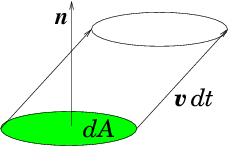
Across any small surface (element) <math xmlns="http://www.w3.org/1998/Math/MathML">
<mrow><mi mathvariant="bold-italic">dA</mi></mrow></math> the flux
(mass per unit time) is equal to <math xmlns="http://www.w3.org/1998/Math/MathML">
<mrow><mi mathvariant="italic">&rho;</mi><mi mathvariant="bold-italic">v</mi><mo>.</mo><mi mathvariant="bold-italic">dA</mi></mrow></math>, as
illustrated in Fig.&nbsp;<a href="chap4.xml#fluxdensityl">4.1</a>.

<div class="p"><!----></div>
<a id="tth_fIg4.1">
</a>   <img src="figures/fluxdensity.png" alt="figures/fluxdensity.png" /><a id="fluxdensity">
</a>
  
<div style="text-align:center">Figure 4.1: The elementary volume of fluid crossing a surface element
    <math xmlns="http://www.w3.org/1998/Math/MathML">
<mrow><mi mathvariant="italic">dA</mi></mrow></math> in time element <math xmlns="http://www.w3.org/1998/Math/MathML">
<mrow><mi mathvariant="italic">dt</mi></mrow></math> is <math xmlns="http://www.w3.org/1998/Math/MathML">
<mrow><mi mathvariant="italic">dt</mi><mi mathvariant="bold-italic">v</mi><mo>.</mo>
<mover><mrow><mi mathvariant="bold-italic">n</mi></mrow>
<mo>&Hat;</mo></mover>
<mi mathvariant="italic">dA</mi><mo>=</mo><mi mathvariant="italic">dt</mi><mi mathvariant="bold-italic">v</mi><mo>.</mo><mi mathvariant="bold-italic">dA</mi></mrow></math>. So the mass per unit time is <math xmlns="http://www.w3.org/1998/Math/MathML">
<mrow><mi mathvariant="italic">&rho;</mi><mi mathvariant="bold-italic">v</mi><mo>.</mo><mi mathvariant="bold-italic">dA</mi></mrow></math>.<a id="fluxdensityl">
</a></div>

<div class="p"><!----></div>
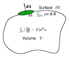
Mass conservation<a 
id="mass_conservation41244"></a> is then described by
considering some control volume <math xmlns="http://www.w3.org/1998/Math/MathML">
<mrow><mi>V</mi></mrow></math> whose surface is <math xmlns="http://www.w3.org/1998/Math/MathML">
<mrow><mo>&part;</mo><mi>V</mi></mrow></math>. For
any such volume, the rate of increase of the total amount of substance
within the volume must be equal to the total source density within the
volume plus the amount flowing in across its surface:
<a id="intconservation">
</a><br />
<table width="100%"><tr><td align="center">
    <math xmlns="http://www.w3.org/1998/Math/MathML">
    <mstyle displaystyle="true"><mrow>
<mfrac><mrow><mo>&part;</mo></mrow>
<mrow><mo>&part;</mo><mi>t</mi></mrow>
</mfrac>

<msub><mrow><mo>&int;</mo></mrow><mrow><mi>V</mi></mrow>
</msub>
<mi mathvariant="italic">&rho;</mi>
<msup><mrow><mi>d</mi></mrow><mrow><mn>3</mn></mrow>
</msup>
<mi>x</mi><mo>=</mo>
<msub><mrow><mo>&int;</mo></mrow><mrow><mi>V</mi></mrow>
</msub>
<mi>S</mi>
<msup><mrow><mi>d</mi></mrow><mrow><mn>3</mn></mrow>
</msup>
<mi>x</mi><mo>-</mo>
<msub><mrow><mo>&int;</mo></mrow><mrow><mo>&part;</mo><mi>V</mi></mrow>
</msub>
<mi mathvariant="italic">&rho;</mi><mi mathvariant="bold-italic">v</mi><mo>.</mo><mi mathvariant="bold-italic">dA</mi><mo>.</mo></mrow>
    </mstyle></math></td><td width="1">
    <math xmlns="http://www.w3.org/1998/Math/MathML">
    <mstyle displaystyle="true"><mrow><mo stretchy="false">(</mo><mn>4</mn><mo>.</mo><mn>2</mn><mo stretchy="false">)</mo></mrow>
    </mstyle></math>
</td></tr></table>


<div class="p"><!----></div>

<div class="p"><!----></div>
<a id="tth_fIg4.2">
</a>   <img src="figures/volumeint.png" alt="figures/volumeint.png" /><a id="volumeint">
</a>
  
<div style="text-align:center">Figure 4.2: Conservation integrals over arbitrary volume <math xmlns="http://www.w3.org/1998/Math/MathML">
<mrow><mi>V</mi></mrow></math> with
    surface <math xmlns="http://www.w3.org/1998/Math/MathML">
<mrow><mo>&part;</mo><mi>V</mi></mrow></math>.<a id="volumeintl">
</a></div>

<div class="p"><!----></div>
Using Gauss's (divergence) theorem<a 
id="Gauss_theorem41245"></a>, illustrated
in Fig.&nbsp;<a href="chap4.xml#volumeintl">4.2</a>, that for any
vector field <math xmlns="http://www.w3.org/1998/Math/MathML">
<mrow><mi mathvariant="bold-italic">u</mi></mrow></math> (here <math xmlns="http://www.w3.org/1998/Math/MathML">
<mrow><mi mathvariant="bold-italic">u</mi><mo>=</mo><mi mathvariant="italic">&rho;</mi><mi mathvariant="bold-italic">v</mi></mrow></math>), the integral over
a closed volume of the divergence is equal to the surface integral of
the vector:
<a id="Gauss">
</a><br />
<table width="100%"><tr><td align="center">
    <math xmlns="http://www.w3.org/1998/Math/MathML">
    <mstyle displaystyle="true"><mrow>
<msub><mrow><mo>&int;</mo></mrow><mrow><mi>V</mi></mrow>
</msub>
<mo>&nabla;</mo><mo>.</mo><mi mathvariant="bold-italic">u</mi><mi>&ensp;&ensp;</mi>
<msup><mrow><mi>d</mi></mrow><mrow><mn>3</mn></mrow>
</msup>
<mi>x</mi><mo>=</mo>
<msub><mrow><mo>&int;</mo></mrow><mrow><mo>&part;</mo><mi>V</mi></mrow>
</msub>
<mi mathvariant="bold-italic">u</mi><mo>.</mo><mi mathvariant="bold-italic">dA</mi><mo>,</mo></mrow>
    </mstyle></math></td><td width="1">
    <math xmlns="http://www.w3.org/1998/Math/MathML">
    <mstyle displaystyle="true"><mrow><mo stretchy="false">(</mo><mn>4</mn><mo>.</mo><mn>3</mn><mo stretchy="false">)</mo></mrow>
    </mstyle></math>
</td></tr></table>


the surface term can be converted to a volume integral and the mass conservation equation becomes:
<a id="preconservation">
</a><br />
<table width="100%"><tr><td align="center">
    <math xmlns="http://www.w3.org/1998/Math/MathML">
    <mstyle displaystyle="true"><mrow>
<msub><mrow><mo>&int;</mo></mrow><mrow><mi>V</mi></mrow>
</msub>
<mrow><mo>(</mo>
<mfrac><mrow><mo>&part;</mo><mi mathvariant="italic">&rho;</mi></mrow>
<mrow><mo>&part;</mo><mi>t</mi></mrow>
</mfrac>
<mo>+</mo><mo>&nabla;</mo><mo>.</mo><mo stretchy="false">(</mo><mi mathvariant="italic">&rho;</mi><mi mathvariant="bold-italic">v</mi><mo stretchy="false">)</mo><mo>-</mo><mi>S</mi><mo>)</mo></mrow>
<msup><mrow><mi>d</mi></mrow><mrow><mn>3</mn></mrow>
</msup>
<mi>x</mi><mo>=</mo><mn>0</mn><mo>.</mo></mrow>
    </mstyle></math></td><td width="1">
    <math xmlns="http://www.w3.org/1998/Math/MathML">
    <mstyle displaystyle="true"><mrow><mo stretchy="false">(</mo><mn>4</mn><mo>.</mo><mn>4</mn><mo stretchy="false">)</mo></mrow>
    </mstyle></math>
</td></tr></table>


This identity applies for <em>any</em> volume <math xmlns="http://www.w3.org/1998/Math/MathML">
<mrow><mi>V</mi></mrow></math>. The only way that can
be true is if the <em>integrand</em> is everywhere equal to zero:
<a id="continuity">
</a><br />
<table width="100%"><tr><td align="center">
    <math xmlns="http://www.w3.org/1998/Math/MathML">
    <mstyle displaystyle="true"><mrow>
<mfrac><mrow><mo>&part;</mo><mi mathvariant="italic">&rho;</mi></mrow>
<mrow><mo>&part;</mo><mi>t</mi></mrow>
</mfrac>
<mo>+</mo><mo>&nabla;</mo><mo>.</mo><mo stretchy="false">(</mo><mi mathvariant="italic">&rho;</mi><mi mathvariant="bold-italic">v</mi><mo stretchy="false">)</mo><mo>-</mo><mi>S</mi><mo>=</mo><mn>0</mn><mo>.</mo></mrow>
    </mstyle></math></td><td width="1">
    <math xmlns="http://www.w3.org/1998/Math/MathML">
    <mstyle displaystyle="true"><mrow><mo stretchy="false">(</mo><mn>4</mn><mo>.</mo><mn>5</mn><mo stretchy="false">)</mo></mrow>
    </mstyle></math>
</td></tr></table>


This is usually called the "continuity" equation. Sometimes,
arguably more physically, it is called the "advection"<a 
id="advection41246"></a> equation. It
is a partial differential equation in three space and one time
variables.

<div class="p"><!----></div>
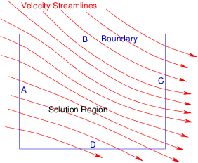
We'll discuss the rest of the fluid equations later; but for now
consider a steady state <math xmlns="http://www.w3.org/1998/Math/MathML">
<mrow>
<mfrac><mrow><mo>&part;</mo></mrow>
<mrow><mo>&part;</mo><mi>t</mi></mrow>
</mfrac>
<mo>=</mo><mn>0</mn></mrow></math>, in which the
velocity <math xmlns="http://www.w3.org/1998/Math/MathML">
<mrow><mi mathvariant="bold-italic">v</mi><mo stretchy="false">(</mo><mi mathvariant="bold-italic">x</mi><mo stretchy="false">)</mo></mrow></math> is prescribed everywhere, illustrated in
Fig. <a href="chap4.xml#advectionl">4.3</a>. The resulting
partial differential equation is
<a id="flow">
</a><br />
<table width="100%"><tr><td align="center">
    <math xmlns="http://www.w3.org/1998/Math/MathML">
    <mstyle displaystyle="true"><mrow><mo>&nabla;</mo><mo>.</mo><mo stretchy="false">(</mo><mi mathvariant="italic">&rho;</mi><mi mathvariant="bold-italic">v</mi><mo stretchy="false">)</mo><mo>=</mo><mi mathvariant="bold-italic">v</mi><mo>.</mo><mo>&nabla;</mo><mi mathvariant="italic">&rho;</mi><mo>+</mo><mi mathvariant="italic">&rho;</mi><mo>&nabla;</mo><mo>.</mo><mi mathvariant="bold-italic">v</mi><mo>=</mo>
<msub><mrow><mi>v</mi></mrow><mrow><mi>x</mi></mrow>
</msub>

<mfrac><mrow><mo>&part;</mo><mi mathvariant="italic">&rho;</mi></mrow>
<mrow><mo>&part;</mo><mi>x</mi></mrow>
</mfrac>
<mo>+</mo>
<msub><mrow><mi>v</mi></mrow><mrow><mi>y</mi></mrow>
</msub>

<mfrac><mrow><mo>&part;</mo><mi mathvariant="italic">&rho;</mi></mrow>
<mrow><mo>&part;</mo><mi>y</mi></mrow>
</mfrac>
<mo>+</mo>
<msub><mrow><mi>v</mi></mrow><mrow><mi>z</mi></mrow>
</msub>

<mfrac><mrow><mo>&part;</mo><mi mathvariant="italic">&rho;</mi></mrow>
<mrow><mo>&part;</mo><mi>z</mi></mrow>
</mfrac>
<mo>+</mo><mi>G</mi><mo stretchy="false">(</mo><mi mathvariant="bold-italic">x</mi><mo stretchy="false">)</mo><mi mathvariant="italic">&rho;</mi><mo>=</mo><mi>S</mi><mo>,</mo></mrow>
    </mstyle></math></td><td width="1">
    <math xmlns="http://www.w3.org/1998/Math/MathML">
    <mstyle displaystyle="true"><mrow><mo stretchy="false">(</mo><mn>4</mn><mo>.</mo><mn>6</mn><mo stretchy="false">)</mo></mrow>
    </mstyle></math>
</td></tr></table>


where the components of the velocity <math xmlns="http://www.w3.org/1998/Math/MathML">
<mrow>
<msub><mrow><mi>v</mi></mrow><mrow><mi>x</mi></mrow>
</msub>
</mrow></math>, <math xmlns="http://www.w3.org/1998/Math/MathML">
<mrow>
<msub><mrow><mi>v</mi></mrow><mrow><mi>y</mi></mrow>
</msub>
</mrow></math>, <math xmlns="http://www.w3.org/1998/Math/MathML">
<mrow>
<msub><mrow><mi>v</mi></mrow><mrow><mi>z</mi></mrow>
</msub>
</mrow></math> and the
divergence of the velocity, <math xmlns="http://www.w3.org/1998/Math/MathML">
<mrow><mi>G</mi><mo>=</mo><mo>&nabla;</mo><mo>.</mo><mi mathvariant="bold-italic">v</mi></mrow></math>, are prescribed
functions of position.
<div class="p"><!----></div>
<a id="tth_fIg4.3">
</a>   <img src="figures/advection.png" alt="figures/advection.png" /><a id="advection">
</a>
  
<div style="text-align:center">Figure 4.3: The advection equation with prescribed velocity <math xmlns="http://www.w3.org/1998/Math/MathML">
<mrow><mi mathvariant="bold-italic">v</mi></mrow></math>
    amounts to integration along the streamlines.  Conditions
    ("initial" conditions) can be applied along the solution region
    boundaries A and B, but not then along C and D.<a id="advectionl">
</a></div>

<div class="p"><!----></div>
From the point of view of solving for <math xmlns="http://www.w3.org/1998/Math/MathML">
<mrow><mi mathvariant="italic">&rho;</mi></mrow></math> as a function of space,
this is a linear first-order partial differential equation in three
dimensions, with variable (i.e. non-uniform) coefficients <math xmlns="http://www.w3.org/1998/Math/MathML">
<mrow>
<msub><mrow><mi>v</mi></mrow><mrow><mi>x</mi></mrow>
</msub>
</mrow></math>,
<math xmlns="http://www.w3.org/1998/Math/MathML">
<mrow>
<msub><mrow><mi>v</mi></mrow><mrow><mi>y</mi></mrow>
</msub>
</mrow></math>, <math xmlns="http://www.w3.org/1998/Math/MathML">
<mrow>
<msub><mrow><mi>v</mi></mrow><mrow><mi>z</mi></mrow>
</msub>
</mrow></math>, and <math xmlns="http://www.w3.org/1998/Math/MathML">
<mrow><mi>G</mi></mrow></math>. It is <em>inhomogeneous</em> if <math xmlns="http://www.w3.org/1998/Math/MathML">
<mrow><mi>S</mi><mo>&ne;</mo><mn>0</mn></mrow></math>, but
<em>homogeneous</em> if <math xmlns="http://www.w3.org/1998/Math/MathML">
<mrow><mi>S</mi><mo>=</mo><mn>0</mn></mrow></math> everywhere.

<div class="p"><!----></div>
     <a id="tth_sEc4.1.2"></a><h3>
4.1.2&nbsp;&nbsp;Diffusion</h3>

<div class="p"><!----></div>
<a 
id="diffusion41247"></a>When a substance such as a gas diffuses through a some other medium,
for example a porous solid, or another (flow free) gas, the flux
density <math xmlns="http://www.w3.org/1998/Math/MathML">
<mrow><mi mathvariant="italic">&rho;</mi><mi mathvariant="bold-italic">v</mi></mrow></math> of the substance is frequently proportional to
the gradient of its density <math xmlns="http://www.w3.org/1998/Math/MathML">
<mrow><mi mathvariant="italic">&rho;</mi></mrow></math>:
<a id="diffusionflux">
</a><br />
<table width="100%"><tr><td align="center">
    <math xmlns="http://www.w3.org/1998/Math/MathML">
    <mstyle displaystyle="true"><mrow><mi mathvariant="italic">&rho;</mi><mi mathvariant="bold-italic">v</mi><mo>=</mo><mo>-</mo><mi>D</mi><mo>&nabla;</mo><mi mathvariant="italic">&rho;</mi><mo>,</mo></mrow>
    </mstyle></math></td><td width="1">
    <math xmlns="http://www.w3.org/1998/Math/MathML">
    <mstyle displaystyle="true"><mrow><mo stretchy="false">(</mo><mn>4</mn><mo>.</mo><mn>7</mn><mo stretchy="false">)</mo></mrow>
    </mstyle></math>
</td></tr></table>


where <math xmlns="http://www.w3.org/1998/Math/MathML">
<mrow><mi>D</mi></mrow></math> is the diffusion coefficient<a 
id="diffusion_coefficient41248"></a>. 

<div class="p"><!----></div>
For such a diffusion problem, we can eliminate the velocity from the
continuity equation (<a href="chap4.xml#continuity">4.5</a>) and obtain the diffusion equation:
<a id="diffusion">
</a><br />
<table width="100%"><tr><td align="center">
    <math xmlns="http://www.w3.org/1998/Math/MathML">
    <mstyle displaystyle="true"><mrow>
<mfrac><mrow><mo>&part;</mo><mi mathvariant="italic">&rho;</mi></mrow>
<mrow><mo>&part;</mo><mi>t</mi></mrow>
</mfrac>
<mo>-</mo><mo>&nabla;</mo><mo>.</mo><mo stretchy="false">(</mo><mi>D</mi><mo>&nabla;</mo><mi mathvariant="italic">&rho;</mi><mo stretchy="false">)</mo><mo>-</mo><mi>S</mi><mo>=</mo><mn>0</mn><mo>.</mo></mrow>
    </mstyle></math></td><td width="1">
    <math xmlns="http://www.w3.org/1998/Math/MathML">
    <mstyle displaystyle="true"><mrow><mo stretchy="false">(</mo><mn>4</mn><mo>.</mo><mn>8</mn><mo stretchy="false">)</mo></mrow>
    </mstyle></math>
</td></tr></table>


This is a linear partial differential equation that is second order in the
spatial derivatives (e.g.&nbsp;if <math xmlns="http://www.w3.org/1998/Math/MathML">
<mrow><mi>D</mi></mrow></math> is uniform the second term becomes
Laplacian <math xmlns="http://www.w3.org/1998/Math/MathML">
<mrow><mo>-</mo><mi>D</mi>
<msup><mrow><mo>&nabla;</mo></mrow><mrow><mn>2</mn></mrow>
</msup>
<mi mathvariant="italic">&rho;</mi></mrow></math>); but it is first order in
time.<a 
id="diffusion_equation41249"></a>

<div class="p"><!----></div>
     <a id="tth_sEc4.1.3"></a><h3>
4.1.3&nbsp;&nbsp;Waves</h3>

<div class="p"><!----></div>
The equation that governs waves in one dimension, for example
small-amplitude compressional vibrations of a column of air in a pipe,
or transverse vibrations of a stretched string or a rigid rod, is
<a id="waveequation">
</a><br />
<table width="100%"><tr><td align="center">
    <math xmlns="http://www.w3.org/1998/Math/MathML">
    <mstyle displaystyle="true"><mrow>
<mfrac><mrow>
<msup><mrow><mo>&part;</mo></mrow><mrow><mn>2</mn></mrow>
</msup>
<mi mathvariant="italic">&psi;</mi></mrow>
<mrow><mo>&part;</mo>
<msup><mrow><mi>t</mi></mrow><mrow><mn>2</mn></mrow>
</msup>
</mrow>
</mfrac>
<mo>=</mo>
<msubsup><mrow><mi>c</mi></mrow><mrow><mi>s</mi> </mrow>
<mrow><mn>2</mn></mrow></msubsup>

<mfrac><mrow>
<msup><mrow><mo>&part;</mo></mrow><mrow><mn>2</mn></mrow>
</msup>
<mi mathvariant="italic">&psi;</mi></mrow>
<mrow><mo>&part;</mo>
<msup><mrow><mi>x</mi></mrow><mrow><mn>2</mn></mrow>
</msup>
</mrow>
</mfrac>
<mo>,</mo></mrow>
    </mstyle></math></td><td width="1">
    <math xmlns="http://www.w3.org/1998/Math/MathML">
    <mstyle displaystyle="true"><mrow><mo stretchy="false">(</mo><mn>4</mn><mo>.</mo><mn>9</mn><mo stretchy="false">)</mo></mrow>
    </mstyle></math>
</td></tr></table>


where <math xmlns="http://www.w3.org/1998/Math/MathML">
<mrow>
<msub><mrow><mi>c</mi></mrow><mrow><mi>s</mi></mrow>
</msub>
</mrow></math> is the wave (sound) speed, and <math xmlns="http://www.w3.org/1998/Math/MathML">
<mrow><mi mathvariant="italic">&psi;</mi></mrow></math> represents the wave
displacement or perturbed quantity (e.g.&nbsp;pressure). The wave
equation<a 
id="wave_equation41250"></a> is second
order in space and time, and linear (provided <math xmlns="http://www.w3.org/1998/Math/MathML">
<mrow>
<msub><mrow><mi>c</mi></mrow><mrow><mi>s</mi></mrow>
</msub>
</mrow></math> does not depend on <math xmlns="http://www.w3.org/1998/Math/MathML">
<mrow><mi mathvariant="italic">&psi;</mi></mrow></math>).

<div class="p"><!----></div>
     <a id="tth_sEc4.1.4"></a><h3>
4.1.4&nbsp;&nbsp;Electromagnetism</h3>

<div class="p"><!----></div>
Maxwell's equations<a 
id="Maxwell_s_equations41251"></a> of electromagnetism, relating the electric<a 
id="electric_field41252"></a> and
magnetic fields<a 
id="magnetic_field41253"></a> <math xmlns="http://www.w3.org/1998/Math/MathML">
<mrow><mi mathvariant="bold-italic">E</mi></mrow></math>, and <math xmlns="http://www.w3.org/1998/Math/MathML">
<mrow><mi mathvariant="bold-italic">B</mi></mrow></math>, to the
charge density<a 
id="charge_density41254"></a>
<math xmlns="http://www.w3.org/1998/Math/MathML">
<mrow>
<msub><mrow><mi mathvariant="italic">&rho;</mi></mrow><mrow><mi>q</mi></mrow>
</msub>
</mrow></math>, and the electric current density<a 
id="current_density41255"></a> <math xmlns="http://www.w3.org/1998/Math/MathML">
<mrow><mi mathvariant="bold-italic">j</mi></mrow></math>, in the absence
of dielectric or magnetic materials are:
<a id="maxwell">
</a><br />
<table width="100%"><tr><td align="center">
    <math xmlns="http://www.w3.org/1998/Math/MathML">
    <mstyle displaystyle="true"><mrow>
<mtable displaystyle="true" align="right" width="80%">
<mtr><mtd columnalign="right" columnspan="1"><mrow></mrow>
</mtd><mtd columnalign="left">
<mrow></mrow>
</mtd><mtd columnalign="left">
<mrow><mo>&nabla;</mo><mo>.</mo><mi mathvariant="bold-italic">E</mi><mo>=</mo>
<msub><mrow><mi mathvariant="italic">&rho;</mi></mrow><mrow><mi>q</mi></mrow>
</msub>
<mo stretchy="false">/</mo>
<msub><mrow><mi mathvariant="italic">&epsi;</mi></mrow><mrow><mn>0</mn></mrow>
</msub>
</mrow>
</mtd><mtd columnalign="right">&emsp;&emsp;&emsp;&emsp;&emsp;&emsp;<mo stretchy="false">(</mo><mn>4</mn><mo>.</mo><mn>10</mn><mo stretchy="false">)</mo></mtd></mtr>
<mtr><mtd columnalign="right" columnspan="1"><mrow></mrow>
</mtd><mtd columnalign="left">
<mrow></mrow>
</mtd><mtd columnalign="left">
<mrow><mo>&nabla;</mo><mo>&times;</mo><mi mathvariant="bold-italic">E</mi><mo>=</mo><mo>-</mo>
<mfrac><mrow><mo>&part;</mo><mi mathvariant="bold-italic">B</mi></mrow>
<mrow><mo>&part;</mo><mi>t</mi></mrow>
</mfrac>
</mrow>
</mtd></mtr>
<mtr><mtd columnalign="right" columnspan="1"><mrow></mrow>
</mtd><mtd columnalign="left">
<mrow></mrow>
</mtd><mtd columnalign="left">
<mrow><mo>&nabla;</mo><mo>.</mo><mi mathvariant="bold-italic">B</mi><mo>=</mo><mn>0</mn></mrow>
</mtd></mtr>
<mtr><mtd columnalign="right" columnspan="1"><mrow></mrow>
</mtd><mtd columnalign="left">
<mrow></mrow>
</mtd><mtd columnalign="left">
<mrow><mo>&nabla;</mo><mo>&times;</mo><mi mathvariant="bold-italic">B</mi><mo>=</mo>
<msub><mrow><mi mathvariant="italic">&mu;</mi></mrow><mrow><mn>0</mn></mrow>
</msub>
<mi mathvariant="bold-italic">j</mi><mo>+</mo>
<msub><mrow><mi mathvariant="italic">&mu;</mi></mrow><mrow><mn>0</mn></mrow>
</msub>

<msub><mrow><mi mathvariant="italic">&epsi;</mi></mrow><mrow><mn>0</mn></mrow>
</msub>

<mfrac><mrow><mo>&part;</mo><mi mathvariant="bold-italic">E</mi></mrow>
<mrow><mo>&part;</mo><mi>t</mi></mrow>
</mfrac>
</mrow>
</mtd></mtr>
</mtable>
</mrow>
    </mstyle></math>
</td></tr></table>
<br />

where <math xmlns="http://www.w3.org/1998/Math/MathML">
<mrow>
<msub><mrow><mi mathvariant="italic">&epsi;</mi></mrow><mrow><mn>0</mn></mrow>
</msub>
<mo>=</mo><mn>8</mn><mo>.</mo><mn>85</mn><mo>&times;</mo>
<msup><mrow><mn>10</mn></mrow><mrow><mo>-</mo><mn>12</mn></mrow>
</msup>
</mrow></math> F/m is the permittivity<a 
id="permittivity41256"></a> of free
space, <math xmlns="http://www.w3.org/1998/Math/MathML">
<mrow>
<msub><mrow><mi mathvariant="italic">&mu;</mi></mrow><mrow><mn>0</mn></mrow>
</msub>
<mo>=</mo><mn>4</mn><mi mathvariant="italic">&pi;</mi><mo>&times;</mo>
<msup><mrow><mn>10</mn></mrow><mrow><mo>-</mo><mn>7</mn></mrow>
</msup>
</mrow></math> H/m is the permeability<a 
id="permeability41257"></a> of free
space. These fundamental constants satisfy <math xmlns="http://www.w3.org/1998/Math/MathML">
<mrow>
<msub><mrow><mi mathvariant="italic">&mu;</mi></mrow><mrow><mn>0</mn></mrow>
</msub>

<msub><mrow><mi mathvariant="italic">&epsi;</mi></mrow><mrow><mn>0</mn></mrow>
</msub>
<mo>=</mo><mn>1</mn><mo stretchy="false">/</mo>
<msup><mrow><mi>c</mi></mrow><mrow><mn>2</mn></mrow>
</msup>
</mrow></math>, where <math xmlns="http://www.w3.org/1998/Math/MathML">
<mrow><mi>c</mi></mrow></math> is the speed of light<a 
id="speed_of_light41258"></a>.

<div class="p"><!----></div>
These are a system of partial differential equations. There appear to
be eight in all because the curl<a 
id="curl41259"></a> equations are vector equations (three
equations in one) and the divergence equations are single equations.
However, there's some built-in redundancy in the equations that
reduces there effective number to six (equal to the number of dependent
variables in the components of the electric and magnetic fields).

<div class="p"><!----></div>
Only rarely does one solve the full set of equations numerically. More
usually one is interested in simplified special cases. For example, if
time dependence can be ignored, then <math xmlns="http://www.w3.org/1998/Math/MathML">
<mrow><mo>&nabla;</mo><mo>&times;</mo><mi mathvariant="bold-italic">E</mi><mo>=</mo><mn>0</mn></mrow></math>, which
is a sufficient condition to allow the electric field to be expressed
as the gradient of a scalar potential <math xmlns="http://www.w3.org/1998/Math/MathML">
<mrow><mi mathvariant="bold-italic">E</mi><mo>=</mo><mo>-</mo><mo>&nabla;</mo><mi mathvariant="italic">&phi;</mi></mrow></math>. In that
case, the potential satisfies<a 
id="electrostatic41260"></a> 
<a id="Poisson">
</a><br />
<table width="100%"><tr><td align="center">
    <math xmlns="http://www.w3.org/1998/Math/MathML">
    <mstyle displaystyle="true"><mrow><mo>-</mo><mo>&nabla;</mo><mo>.</mo><mi mathvariant="bold-italic">E</mi><mo>=</mo><mo>-</mo><mo>&nabla;</mo><mo>.</mo><mo stretchy="false">(</mo><mo>-</mo><mo>&nabla;</mo><mi mathvariant="italic">&phi;</mi><mo stretchy="false">)</mo><mo>=</mo>
<msup><mrow><mo>&nabla;</mo></mrow><mrow><mn>2</mn></mrow>
</msup>
<mi mathvariant="italic">&phi;</mi><mo>=</mo>
<mfrac><mrow>
<msup><mrow><mo>&part;</mo></mrow><mrow><mn>2</mn></mrow>
</msup>
<mi mathvariant="italic">&phi;</mi></mrow>
<mrow><mo>&part;</mo>
<msup><mrow><mi>x</mi></mrow><mrow><mn>2</mn></mrow>
</msup>
</mrow>
</mfrac>
<mo>+</mo>
<mfrac><mrow>
<msup><mrow><mo>&part;</mo></mrow><mrow><mn>2</mn></mrow>
</msup>
<mi mathvariant="italic">&phi;</mi></mrow>
<mrow><mo>&part;</mo>
<msup><mrow><mi>y</mi></mrow><mrow><mn>2</mn></mrow>
</msup>
</mrow>
</mfrac>
<mo>+</mo>
<mfrac><mrow>
<msup><mrow><mo>&part;</mo></mrow><mrow><mn>2</mn></mrow>
</msup>
<mi mathvariant="italic">&phi;</mi></mrow>
<mrow><mo>&part;</mo>
<msup><mrow><mi>z</mi></mrow><mrow><mn>2</mn></mrow>
</msup>
</mrow>
</mfrac>
<mo>=</mo><mo>-</mo>
<msub><mrow><mi mathvariant="italic">&rho;</mi></mrow><mrow><mi>q</mi></mrow>
</msub>
<mo stretchy="false">/</mo>
<msub><mrow><mi mathvariant="italic">&epsi;</mi></mrow><mrow><mn>0</mn></mrow>
</msub>
<mo>,</mo></mrow>
    </mstyle></math></td><td width="1">
    <math xmlns="http://www.w3.org/1998/Math/MathML">
    <mstyle displaystyle="true"><mrow><mo stretchy="false">(</mo><mn>4</mn><mo>.</mo><mn>11</mn><mo stretchy="false">)</mo></mrow>
    </mstyle></math>
</td></tr></table>


which is Poisson's equation<a href="footnote.xml#tthFtNtACD" id="tthFrefACD"><math xmlns="http://www.w3.org/1998/Math/MathML">
<mrow>
<msup><mrow></mrow><mrow><mn>23</mn></mrow>
</msup>
</mrow></math></a><a 
id="Poisson_equation41261"></a>. Poisson's equation sets a <em>second
  order</em> differential, the <em>Laplacian</em><a 
id="Laplacian41262"></a> (<math xmlns="http://www.w3.org/1998/Math/MathML">
<mrow>
<msup><mrow><mo>&nabla;</mo></mrow><mrow><mn>2</mn></mrow>
</msup>
</mrow></math>) of the
potential equal to a (presumably prescribed) function <math xmlns="http://www.w3.org/1998/Math/MathML">
<mrow><mo>-</mo>
<msub><mrow><mi mathvariant="italic">&rho;</mi></mrow><mrow><mi>q</mi></mrow>
</msub>
<mo stretchy="false">/</mo>
<msub><mrow><mi mathvariant="italic">&epsi;</mi></mrow><mrow><mn>0</mn></mrow>
</msub>
</mrow></math>.

<div class="p"><!----></div>
 <a id="tth_sEc4.2"></a><h2>
4.2&nbsp;&nbsp;Classification of Partial Differential Equations</h2>

<div class="p"><!----></div>
<a 
id="PDE_classification42263"></a><a 
id="classification_of_PDEs42264"></a> In the theory
of partial differential equations, there are three types of
differential equation. They are called: Hyperbolic<a 
id="hyperbolic42265"></a>,
Parabolic<a 
id="parabolic42266"></a>, and Elliptic<a 
id="elliptic42267"></a>. To
understand this classification rigorously would take us far beyond our
scope, but it is important for computation because the methods of
solving the different types of equation are different.

<div class="p"><!----></div>
For our purposes, the classification can be considered
as follows for second order equations. Write the general linear
second-order partial differential equation governing dependent
variable <math xmlns="http://www.w3.org/1998/Math/MathML">
<mrow><mi mathvariant="italic">&psi;</mi></mrow></math> for independent variables <math xmlns="http://www.w3.org/1998/Math/MathML">
<mrow>
<msub><mrow><mi>x</mi></mrow><mrow><mi>i</mi></mrow>
</msub>
</mrow></math> as
<a id="general2nd">
</a><br />
<table width="100%"><tr><td align="center">
    <math xmlns="http://www.w3.org/1998/Math/MathML">
    <mstyle displaystyle="true"><mrow>
<munder><mo>&sum;</mo><mrow><mi>i</mi><mo>,</mo><mi>j</mi></mrow>
</munder>

<msub><mrow><mi>c</mi></mrow><mrow><mi mathvariant="italic">ij</mi></mrow>
</msub>

<mfrac><mrow><mo>&part;</mo></mrow>
<mrow><mo>&part;</mo>
<msub><mrow><mi>x</mi></mrow><mrow><mi>i</mi></mrow>
</msub>
</mrow>
</mfrac>

<mfrac><mrow><mo>&part;</mo></mrow>
<mrow><mo>&part;</mo>
<msub><mrow><mi>x</mi></mrow><mrow><mi>j</mi></mrow>
</msub>
</mrow>
</mfrac>
<mi mathvariant="italic">&psi;</mi><mo>+</mo>
<munder><mo>&sum;</mo><mrow><mi>i</mi></mrow>
</munder>

<msub><mrow><mi>c</mi></mrow><mrow><mi>i</mi></mrow>
</msub>

<mfrac><mrow><mo>&part;</mo></mrow>
<mrow><mo>&part;</mo>
<msub><mrow><mi>x</mi></mrow><mrow><mi>i</mi></mrow>
</msub>
</mrow>
</mfrac>
<mi mathvariant="italic">&psi;</mi><mo>+</mo><mi>c</mi><mi mathvariant="italic">&psi;</mi><mo>=</mo><mi mathvariant="italic">const</mi><mo>.</mo></mrow>
    </mstyle></math></td><td width="1">
    <math xmlns="http://www.w3.org/1998/Math/MathML">
    <mstyle displaystyle="true"><mrow><mo stretchy="false">(</mo><mn>4</mn><mo>.</mo><mn>12</mn><mo stretchy="false">)</mo></mrow>
    </mstyle></math>
</td></tr></table>


A specific example might be 
<a id="specific2nd">
</a><br />
<table width="100%"><tr><td align="center">
    <math xmlns="http://www.w3.org/1998/Math/MathML">
    <mstyle displaystyle="true"><mrow><mi>A</mi>
<mfrac><mrow>
<msup><mrow><mo>&part;</mo></mrow><mrow><mn>2</mn></mrow>
</msup>
</mrow>
<mrow><mo>&part;</mo>
<msup><mrow><mi>x</mi></mrow><mrow><mn>2</mn></mrow>
</msup>
</mrow>
</mfrac>
<mi mathvariant="italic">&psi;</mi><mo>+</mo><mn>2</mn><mi>B</mi>
<mfrac><mrow>
<msup><mrow><mo>&part;</mo></mrow><mrow><mn>2</mn></mrow>
</msup>
</mrow>
<mrow><mo>&part;</mo><mi>x</mi><mo>&part;</mo><mi>y</mi></mrow>
</mfrac>
<mi mathvariant="italic">&psi;</mi><mo>+</mo><mi>C</mi>
<mfrac><mrow>
<msup><mrow><mo>&part;</mo></mrow><mrow><mn>2</mn></mrow>
</msup>
</mrow>
<mrow><mo>&part;</mo>
<msup><mrow><mi>y</mi></mrow><mrow><mn>2</mn></mrow>
</msup>
</mrow>
</mfrac>
<mi mathvariant="italic">&psi;</mi><mo>=</mo><mn>0</mn><mo>.</mo></mrow>
    </mstyle></math></td><td width="1">
    <math xmlns="http://www.w3.org/1998/Math/MathML">
    <mstyle displaystyle="true"><mrow><mo stretchy="false">(</mo><mn>4</mn><mo>.</mo><mn>13</mn><mo stretchy="false">)</mo></mrow>
    </mstyle></math>
</td></tr></table>


Consider the coefficients <math xmlns="http://www.w3.org/1998/Math/MathML">
<mrow>
<msub><mrow><mi>c</mi></mrow><mrow><mi mathvariant="italic">ij</mi></mrow>
</msub>
</mrow></math>, and regard them as defining a
surface in the multidimensional space via the quadratic
form<a 
id="quadratic_form42268"></a> associated with them:
<a id="genquadform">
</a><br />
<table width="100%"><tr><td align="center">
    <math xmlns="http://www.w3.org/1998/Math/MathML">
    <mstyle displaystyle="true"><mrow>
<munder><mo>&sum;</mo><mrow><mi>i</mi><mo>,</mo><mi>j</mi></mrow>
</munder>

<msub><mrow><mi>c</mi></mrow><mrow><mi mathvariant="italic">ij</mi></mrow>
</msub>

<msub><mrow><mi>x</mi></mrow><mrow><mi>i</mi></mrow>
</msub>

<msub><mrow><mi>x</mi></mrow><mrow><mi>j</mi></mrow>
</msub>
<mo>+</mo>
<munder><mo>&sum;</mo><mrow><mi>i</mi></mrow>
</munder>

<msub><mrow><mi>c</mi></mrow><mrow><mi>i</mi></mrow>
</msub>

<msub><mrow><mi>x</mi></mrow><mrow><mi>i</mi></mrow>
</msub>
<mo>=</mo><mi mathvariant="italic">const</mi><mo>.</mo></mrow>
    </mstyle></math></td><td width="1">
    <math xmlns="http://www.w3.org/1998/Math/MathML">
    <mstyle displaystyle="true"><mrow><mo stretchy="false">(</mo><mn>4</mn><mo>.</mo><mn>14</mn><mo stretchy="false">)</mo></mrow>
    </mstyle></math>
</td></tr></table>


Specifically:
<a id="specquadform">
</a><br />
<table width="100%"><tr><td align="center">
    <math xmlns="http://www.w3.org/1998/Math/MathML">
    <mstyle displaystyle="true"><mrow>
<msup><mrow><mi mathvariant="italic">Ax</mi></mrow><mrow><mn>2</mn></mrow>
</msup>
<mo>+</mo><mn>2</mn><mi>B</mi><mi mathvariant="italic">xy</mi><mo>+</mo>
<msup><mrow><mi mathvariant="italic">Cy</mi></mrow><mrow><mn>2</mn></mrow>
</msup>
<mo>=</mo><mi mathvariant="italic">const</mi><mo>.</mo></mrow>
    </mstyle></math></td><td width="1">
    <math xmlns="http://www.w3.org/1998/Math/MathML">
    <mstyle displaystyle="true"><mrow><mo stretchy="false">(</mo><mn>4</mn><mo>.</mo><mn>15</mn><mo stretchy="false">)</mo></mrow>
    </mstyle></math>
</td></tr></table>


Then the partial differential equation is hyperbolic,
  parabolic, or elliptic according to whether the surface so defined
  is itself hyperbolic, parabolic, or elliptic.

<div class="p"><!----></div>
For our two-dimensional specific example, the surface is 

<dl>
 <dt><b>Hyperbolic</b></dt>
	<dd> if <math xmlns="http://www.w3.org/1998/Math/MathML">
<mrow>
<msup><mrow><mi>B</mi></mrow><mrow><mn>2</mn></mrow>
</msup>
<mo>-</mo><mi mathvariant="italic">AC</mi><mo>&gt;</mo><mn>0</mn></mrow></math>; for example <math xmlns="http://www.w3.org/1998/Math/MathML">
<mrow><mi>B</mi><mo>=</mo><mn>0</mn></mrow></math>, <math xmlns="http://www.w3.org/1998/Math/MathML">
<mrow><mi>C</mi><mo>=</mo><mo>-</mo><mi>A</mi></mrow></math>, <math xmlns="http://www.w3.org/1998/Math/MathML">
<mrow>
<msup><mrow><mi>x</mi></mrow><mrow><mn>2</mn></mrow>
</msup>
<mo>-</mo>
<msup><mrow><mi>y</mi></mrow><mrow><mn>2</mn></mrow>
</msup>
<mo>=</mo><mi mathvariant="italic">const</mi><mo>.</mo></mrow></math></dd>
 <dt><b>Parabolic</b></dt>
	<dd> if  <math xmlns="http://www.w3.org/1998/Math/MathML">
<mrow>
<msup><mrow><mi>B</mi></mrow><mrow><mn>2</mn></mrow>
</msup>
<mo>-</mo><mi mathvariant="italic">AC</mi><mo>=</mo><mn>0</mn></mrow></math>; for example <math xmlns="http://www.w3.org/1998/Math/MathML">
<mrow><mi>B</mi><mo>=</mo><mi>C</mi><mo>=</mo><mn>0</mn></mrow></math>, <math xmlns="http://www.w3.org/1998/Math/MathML">
<mrow>
<msup><mrow><mi>x</mi></mrow><mrow><mn>2</mn></mrow>
</msup>
<mo>-</mo><mi>y</mi><mo>=</mo><mi mathvariant="italic">const</mi><mo>.</mo></mrow></math></dd>
 <dt><b>Elliptic</b></dt>
	<dd> if  <math xmlns="http://www.w3.org/1998/Math/MathML">
<mrow>
<msup><mrow><mi>B</mi></mrow><mrow><mn>2</mn></mrow>
</msup>
<mo>-</mo><mi mathvariant="italic">AC</mi><mo>&lt;</mo><mn>0</mn></mrow></math>; for example <math xmlns="http://www.w3.org/1998/Math/MathML">
<mrow><mi>B</mi><mo>=</mo><mn>0</mn></mrow></math>, <math xmlns="http://www.w3.org/1998/Math/MathML">
<mrow><mi>C</mi><mo>=</mo><mi>A</mi></mrow></math>, <math xmlns="http://www.w3.org/1998/Math/MathML">
<mrow>
<msup><mrow><mi>x</mi></mrow><mrow><mn>2</mn></mrow>
</msup>
<mo>+</mo>
<msup><mrow><mi>y</mi></mrow><mrow><mn>2</mn></mrow>
</msup>
<mo>=</mo><mi mathvariant="italic">const</mi><mo>.</mo></mrow></math></dd>
</dl>
And so is the equation.
The examples we have given previously illustrate characteristically
these different types. 

<div class="p"><!----></div>
The <i>wave equation</i> is <i>hyperbolic</i>.

<div class="p"><!----></div>
The <i>diffusion equation</i> is <i>parabolic</i>.

<div class="p"><!----></div>
The <i>Poisson equation</i> is <i>elliptic</i>.

<div class="p"><!----></div>
The first order equation for fluid flow with prescribed velocity
(advection equation) is ambiguous under this classification because
the surface for a first order form is a plane. But a plane can be
considered a degenerate hyperbola, because it extends to infinity
(unlike an ellipse which is finite in extent). The first order
system for one scalar dependent variable is always
hyperbolic.<a href="footnote.xml#tthFtNtACE" id="tthFrefACE"><math xmlns="http://www.w3.org/1998/Math/MathML">
<mrow>
<msup><mrow></mrow><mrow><mn>24</mn></mrow>
</msup>
</mrow></math></a>

<div class="p"><!----></div>
Loosely speaking, second order hyperbolic equations are wave-like, and
elliptic equations are steady-flux-conservation-like. A hyperbolic
or parabolic equation generally has at least one independent variable
that is like time, as well as others that are like space. An
elliptic problem is more like a steady (non-time-varying) problem in
multiple space dimensions. The classification is more fundamentally to
do with whether a problem of order <math xmlns="http://www.w3.org/1998/Math/MathML">
<mrow><mi>N</mi></mrow></math> with <math xmlns="http://www.w3.org/1998/Math/MathML">
<mrow><mi>N</mi></mrow></math> boundary
conditions<a 
id="boundary_condition42269"></a> on a single surface (the
multidimensional equivalent of an initial value problem) can be solved
or not. Such a problem is called a Cauchy problem<a 
id="Cauchy_problem42270"></a>.
Generally, hyperbolic equations are those for which the
Cauchy problem can be solved; for elliptic equations it cannot.

<div class="p"><!----></div>
The most important distinction from the viewpoint of numerical
solution of partial differential equations is with respect to the
boundary conditions. Are these all applied on a single open surface,
such as the plane at <math xmlns="http://www.w3.org/1998/Math/MathML">
<mrow><mi>t</mi><mo>=</mo><mn>0</mn></mrow></math>? If so (hyperbolic and parabolic equations
only) then this is an <em>initial value problem</em> where we are trying
to solve for the time evolution and we can integrate forward in time
from the initial conditions. For example, recalling Fig.&nbsp;<a href="chap4.xml#advectionl">4.3</a> for the (hyperbolic) advection<a 
id="advection42271"></a>
equation, one can see immediately that because the equation governs
the variation of density along a streamline, it could make no sense to
apply conditions at two different points along the one
streamline<a 
id="streamline42272"></a>.

<div class="p"><!----></div>
<a id="tth_fIg4.4">
</a>   <img src="figures/ellipBC.png" alt="figures/ellipBC.png" /><a id="ellipBC">
</a>
  
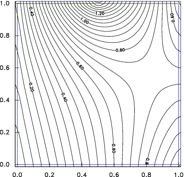
<div style="text-align:center">Figure 4.4: An elliptic equation, such as Laplace's equation has
    boundary conditions applied round an entire closed surface. In
    this case, the potential is prescribed everywhere on the square
    domain boundary, and contours of potential are plotted.<a id="ellipBCl">
</a></div>

<div class="p"><!----></div>
Alternatively, are the conditions applied on the boundary of a closed
domain (as illustrated in Fig.&nbsp;<a href="chap4.xml#ellipBCl">4.4</a>)? If so (elliptic
equations) then the solution everywhere depends upon all the boundary
information, it is called a <em>boundary value
  problem</em><a 
id="boundary_value_problem42273"></a>. Then we generally can't
successfully integrate from the boundary. "Shooting" doesn't work in
multiple dimensions; so we can't turn the problem into an interative
initial value problem the way we did in one-dimension. We have to
converge to the full solution everywhere simultaneously.

<div class="p"><!----></div>
 <a id="tth_sEc4.3"></a><h2>
4.3&nbsp;&nbsp;Finite Difference Partial Derivatives</h2>

<div class="p"><!----></div>
As with ordinary differential equations, a key step in implementing
numerical solution of partial differential equations is the expression
of the derivatives in terms of the discrete numerical representation
of the variables<a 
id="discrete_representation43274"></a>. There are many
possible such discrete representations. One might be in terms of the
Fourier coefficients <math xmlns="http://www.w3.org/1998/Math/MathML">
<mrow>
<msub><mrow><mi>a</mi></mrow><mrow><mi mathvariant="italic">ij</mi></mrow>
</msub>
</mrow></math> of a discrete Fourier representation
such as<a 
id="Fourier_representation43275"></a>:
<a id="fourierrep">
</a><br />
<table width="100%"><tr><td align="center">
    <math xmlns="http://www.w3.org/1998/Math/MathML">
    <mstyle displaystyle="true"><mrow><mi mathvariant="italic">&psi;</mi><mo>=</mo>
<munder><mo>&sum;</mo><mrow><mi>i</mi><mo>,</mo><mi>j</mi></mrow>
</munder>

<msub><mrow><mi>a</mi></mrow><mrow><mi mathvariant="italic">ij</mi></mrow>
</msub>
<mi>sin</mi><mo stretchy="false">(</mo><mi mathvariant="italic">&pi;</mi><mi>i</mi><mi>x</mi><mo stretchy="false">/</mo>
<msub><mrow><mi>L</mi></mrow><mrow><mi>x</mi></mrow>
</msub>
<mo stretchy="false">)</mo><mi>sin</mi><mo stretchy="false">(</mo><mi mathvariant="italic">&pi;</mi><mi>j</mi><mi>y</mi><mo stretchy="false">/</mo>
<msub><mrow><mi>L</mi></mrow><mrow><mi>y</mi></mrow>
</msub>
<mo stretchy="false">)</mo><mo>,</mo></mrow>
    </mstyle></math></td><td width="1">
    <math xmlns="http://www.w3.org/1998/Math/MathML">
    <mstyle displaystyle="true"><mrow><mo stretchy="false">(</mo><mn>4</mn><mo>.</mo><mn>16</mn><mo stretchy="false">)</mo></mrow>
    </mstyle></math>
</td></tr></table>


(where we've chosen to rule out cosine terms by presuming the boundary
conditions to be <math xmlns="http://www.w3.org/1998/Math/MathML">
<mrow><mi mathvariant="italic">&psi;</mi><mo>=</mo><mn>0</mn></mrow></math> at <math xmlns="http://www.w3.org/1998/Math/MathML">
<mrow><mi>x</mi><mo>=</mo><mn>0</mn><mo>,</mo>
<msub><mrow><mi>L</mi></mrow><mrow><mi>x</mi></mrow>
</msub>
</mrow></math> or <math xmlns="http://www.w3.org/1998/Math/MathML">
<mrow><mi>y</mi><mo>=</mo><mn>0</mn><mo>,</mo>
<msub><mrow><mi>L</mi></mrow><mrow><mi>y</mi></mrow>
</msub>
</mrow></math>). There are some
equations in which it is computationally efficient to work in terms of
such coefficients, especially in coordinate directions that are ignorable. 
Far more often, though, the representation of our variables is on a
discrete spatial mesh with finite spacing in the independent
variables.

<div class="p"><!----></div>
A mesh is considered to be "structured"<a 
id="structured_mesh43276"></a> if
the points at which the solution is to be found are in a regular order
in each of the coordinate directions. The most obvious choice is
cartesian<a 
id="cartesian43277"></a> coordinates. The mesh nodes would then be
at positions <math xmlns="http://www.w3.org/1998/Math/MathML">
<mrow><mo stretchy="false">(</mo>
<msub><mrow><mi>x</mi></mrow><mrow><mi>n</mi></mrow>
</msub>
<mo>,</mo>
<msub><mrow><mi>y</mi></mrow><mrow><mi>m</mi></mrow>
</msub>
<mo>,</mo>
<msub><mrow><mi>z</mi></mrow><mrow><mi>l</mi></mrow>
</msub>
<mo stretchy="false">)</mo></mrow></math>, where each array <math xmlns="http://www.w3.org/1998/Math/MathML">
<mrow>
<msub><mrow><mi>x</mi></mrow><mrow><mi>n</mi></mrow>
</msub>
</mrow></math>, <math xmlns="http://www.w3.org/1998/Math/MathML">
<mrow>
<msub><mrow><mi>y</mi></mrow><mrow><mi>m</mi></mrow>
</msub>
</mrow></math>, etc., is
ordered <math xmlns="http://www.w3.org/1998/Math/MathML">
<mrow>
<msub><mrow><mi>x</mi></mrow><mrow><mi>n</mi><mo>-</mo><mn>1</mn></mrow>
</msub>
<mo>&lt;</mo>
<msub><mrow><mi>x</mi></mrow><mrow><mi>n</mi></mrow>
</msub>
<mo>&lt;</mo>
<msub><mrow><mi>x</mi></mrow><mrow><mi>n</mi><mo>+</mo><mn>1</mn></mrow>
</msub>
</mrow></math>, etc. The mesh is then
"uniform"<a 
id="uniform_mesh43278"></a> if the spacing between nodes is the
same for all nodes: <math xmlns="http://www.w3.org/1998/Math/MathML">
<mrow>
<msub><mrow><mi>x</mi></mrow><mrow><mi>n</mi><mo>+</mo><mn>1</mn></mrow>
</msub>
<mo>-</mo>
<msub><mrow><mi>x</mi></mrow><mrow><mi>n</mi></mrow>
</msub>
<mo>=</mo><mi mathvariant="italic">&Delta;</mi><mi>x</mi></mrow></math> for all <math xmlns="http://www.w3.org/1998/Math/MathML">
<mrow><mi>n</mi></mrow></math>, and similarly
for <math xmlns="http://www.w3.org/1998/Math/MathML">
<mrow><mi>y</mi></mrow></math>, <math xmlns="http://www.w3.org/1998/Math/MathML">
<mrow><mi>z</mi></mrow></math>. Structured meshes are also possible on general
curvilinear coordinates<a 
id="curvilinear_coordinates43279"></a>, for example
cylindrical or spherical coordinates, provided the domain remains
"rectangular" in the coordinates; in other words, provided for some
set of coordinates <math xmlns="http://www.w3.org/1998/Math/MathML">
<mrow><mo stretchy="false">(</mo><mi mathvariant="italic">&xi;</mi><mo>,</mo><mi mathvariant="italic">&eta;</mi><mo>,</mo><mi mathvariant="italic">&zeta;</mi><mo stretchy="false">)</mo></mrow></math>, the <math xmlns="http://www.w3.org/1998/Math/MathML">
<mrow>
<msub><mrow><mi mathvariant="italic">&xi;</mi></mrow><mrow><mi>n</mi></mrow>
</msub>
</mrow></math> are independent of
<math xmlns="http://www.w3.org/1998/Math/MathML">
<mrow>
<msub><mrow><mi mathvariant="italic">&eta;</mi></mrow><mrow><mi>m</mi></mrow>
</msub>
</mrow></math> and <math xmlns="http://www.w3.org/1998/Math/MathML">
<mrow>
<msub><mrow><mi mathvariant="italic">&zeta;</mi></mrow><mrow><mi>l</mi></mrow>
</msub>
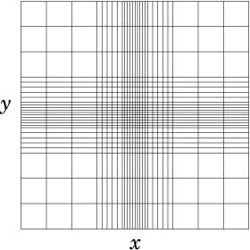
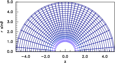
</mrow></math>, and so on. Fig.&nbsp;<a href="chap4.xml#grids">4.5</a> gives two
examples. For such structured meshes, the
most natural and adaptable finite representation is by finite
differences<a 
id="finite_difference43280"></a>.

<div class="p"><!----></div>
<a id="tth_fIg4.5">
</a>  <div style="text-align:center">  <img src="figures/gridrect.png" alt="figures/gridrect.png" /><a id="gridrect">
</a>(a)<img src="figures/gridfig3.png" alt="figures/gridfig3.png" /><a id="gridfig3">
</a>(b)&nbsp;
  
<div style="text-align:center">Figure 4.5: Structured grids. (a) Rectangular, but non-uniform. (b)
    Curvilinear, but still structured.<a id="grids">
</a></div>
</div>
<div class="p"><!----></div>
By contrast, an <em>unstructured</em><a 
id="unstructured_mesh43281"></a> grid can
have any degree of connectedness. Its cells will not generally be
quadrilaterals<a 
id="quadrilateral43282"></a> (in two-dimensions) or
hexahedrons<a 
id="hexahedron43283"></a> (in three dimensions) and it is far less
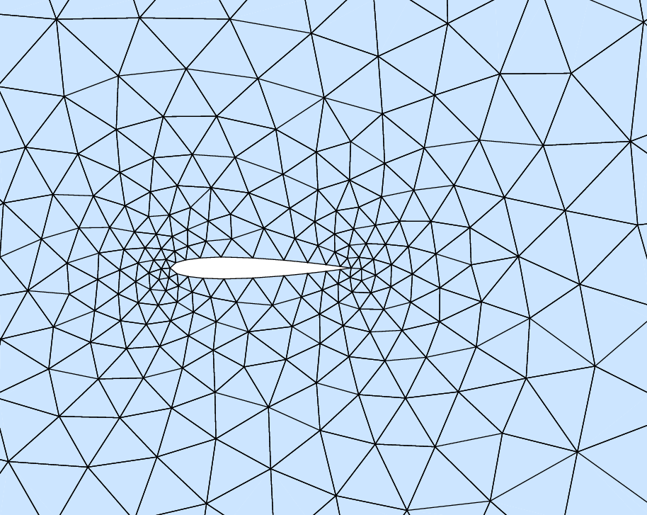
clear how to construct a finite-difference scheme. Fig.&nbsp;<a href="chap4.xml#unstructured">4.6</a> shows an example of a triangular unstructured
mesh<a href="footnote.xml#tthFtNtACF" id="tthFrefACF"><math xmlns="http://www.w3.org/1998/Math/MathML">
<mrow>
<msup><mrow></mrow><mrow><mn>25</mn></mrow>
</msup>
</mrow></math></a>.

<div class="p"><!----></div>
<a id="tth_fIg4.6">
</a>   <img src="figures/airfoil.png" alt="figures/airfoil.png" /><a id="airfoil">
</a>
  
<div style="text-align:center">Figure 4.6: A region of an unstructured mesh. Such meshes are
    designed to give greater resolution in areas of more rapid
    variation, often close to boundaries of complicated or subtle
    shapes. This example uses a triangular mesh but other choices are
    possible.<a id="unstructured">
</a></div>

<div class="p"><!----></div>
We'll stick to structured meshes here.

<div class="p"><!----></div>
Just as in one dimension we use a representation
<a id="diff1d">
</a><br />
<table width="100%"><tr><td align="center">
    <math xmlns="http://www.w3.org/1998/Math/MathML">
    <mstyle displaystyle="true"><mrow>
<msub><mrow><mo> </mo>
<mfrac><mrow><mi>d</mi><mi mathvariant="italic">&psi;</mi></mrow>
<mrow><mi mathvariant="italic">dx</mi></mrow>
</mfrac>
<mo>|</mo></mrow><mrow><mi>n</mi><mo>+</mo><mn>1</mn><mo stretchy="false">/</mo><mn>2</mn></mrow>
</msub>
<mo>=</mo>
<mfrac><mrow>
<msub><mrow><mi mathvariant="italic">&psi;</mi></mrow><mrow><mi>n</mi><mo>+</mo><mn>1</mn></mrow>
</msub>
<mo>-</mo>
<msub><mrow><mi mathvariant="italic">&psi;</mi></mrow><mrow><mi>n</mi></mrow>
</msub>
</mrow>
<mrow>
<msub><mrow><mi>x</mi></mrow><mrow><mi>n</mi><mo>+</mo><mn>1</mn></mrow>
</msub>
<mo>-</mo>
<msub><mrow><mi>x</mi></mrow><mrow><mi>n</mi></mrow>
</msub>
</mrow>
</mfrac>
<mo>,</mo></mrow>
    </mstyle></math></td><td width="1">
    <math xmlns="http://www.w3.org/1998/Math/MathML">
    <mstyle displaystyle="true"><mrow><mo stretchy="false">(</mo><mn>4</mn><mo>.</mo><mn>17</mn><mo stretchy="false">)</mo></mrow>
    </mstyle></math>
</td></tr></table>


so in two dimensions<a 
id="derivative_2-dimensional43284"></a> we can
generalize this to partial derivatives of a dependent variable
<math xmlns="http://www.w3.org/1998/Math/MathML">
<mrow><mi mathvariant="italic">&psi;</mi><mo stretchy="false">(</mo><mi>x</mi><mo>,</mo><mi>y</mi><mo stretchy="false">)</mo></mrow></math> in <math xmlns="http://www.w3.org/1998/Math/MathML">
<mrow><mi>x</mi></mrow></math> and <math xmlns="http://www.w3.org/1998/Math/MathML">
<mrow><mi>y</mi></mrow></math> on mesh positions <math xmlns="http://www.w3.org/1998/Math/MathML">
<mrow><mi>n</mi><mo>,</mo><mi>m</mi></mrow></math> as
<a id="diff2d">
</a><br />
<table width="100%"><tr><td align="center">
    <math xmlns="http://www.w3.org/1998/Math/MathML">
    <mstyle displaystyle="true"><mrow>
<msub><mrow><mo> </mo>
<mfrac><mrow><mo>&part;</mo><mi mathvariant="italic">&psi;</mi></mrow>
<mrow><mo>&part;</mo><mi>x</mi></mrow>
</mfrac>
<mo>|</mo></mrow><mrow><mi>n</mi><mo>+</mo><mn>1</mn><mo stretchy="false">/</mo><mn>2</mn><mo>,</mo><mi>m</mi></mrow>
</msub>
<mo>=</mo>
<mfrac><mrow>
<msub><mrow><mi mathvariant="italic">&psi;</mi></mrow><mrow><mi>n</mi><mo>+</mo><mn>1</mn><mo>,</mo><mi>m</mi></mrow>
</msub>
<mo>-</mo>
<msub><mrow><mi mathvariant="italic">&psi;</mi></mrow><mrow><mi>n</mi><mo>,</mo><mi>m</mi></mrow>
</msub>
</mrow>
<mrow>
<msub><mrow><mi>x</mi></mrow><mrow><mi>n</mi><mo>+</mo><mn>1</mn></mrow>
</msub>
<mo>-</mo>
<msub><mrow><mi>x</mi></mrow><mrow><mi>n</mi></mrow>
</msub>
</mrow>
</mfrac>
<mo>,</mo><mi>&emsp;&emsp;&emsp;&emsp;&emsp;&emsp;</mi>
<msub><mrow><mo> </mo>
<mfrac><mrow><mo>&part;</mo><mi mathvariant="italic">&psi;</mi></mrow>
<mrow><mo>&part;</mo><mi>y</mi></mrow>
</mfrac>
<mo>|</mo></mrow><mrow><mi>n</mi><mo>,</mo><mi>m</mi><mo>+</mo><mn>1</mn><mo stretchy="false">/</mo><mn>2</mn></mrow>
</msub>
<mo>=</mo>
<mfrac><mrow>
<msub><mrow><mi mathvariant="italic">&psi;</mi></mrow><mrow><mi>n</mi><mo>,</mo><mi>m</mi><mo>+</mo><mn>1</mn></mrow>
</msub>
<mo>-</mo>
<msub><mrow><mi mathvariant="italic">&psi;</mi></mrow><mrow><mi>n</mi><mo>,</mo><mi>m</mi></mrow>
</msub>
</mrow>
<mrow>
<msub><mrow><mi>y</mi></mrow><mrow><mi>m</mi><mo>+</mo><mn>1</mn></mrow>
</msub>
<mo>-</mo>
<msub><mrow><mi>y</mi></mrow><mrow><mi>m</mi></mrow>
</msub>
</mrow>
</mfrac>
<mo>,</mo></mrow>
    </mstyle></math></td><td width="1">
    <math xmlns="http://www.w3.org/1998/Math/MathML">
    <mstyle displaystyle="true"><mrow><mo stretchy="false">(</mo><mn>4</mn><mo>.</mo><mn>18</mn><mo stretchy="false">)</mo></mrow>
    </mstyle></math>
</td></tr></table>


with obvious generalization to higher dimensions. Two (or more)
indices denote the mesh node (or half-node position) where the value
of the variable is to be considered evaluated.

<div class="p"><!----></div>
Higher derivatives<a 
id="derivative_higher43285"></a> are formed by taking
appropriate differences of derivative expressions. So
<a id="2ndx">
</a><br />
<table width="100%"><tr><td align="center">
    <math xmlns="http://www.w3.org/1998/Math/MathML">
    <mstyle displaystyle="true"><mrow>
<msub><mrow><mo> </mo>
<mfrac><mrow>
<msup><mrow><mo>&part;</mo></mrow><mrow><mn>2</mn></mrow>
</msup>
<mi mathvariant="italic">&psi;</mi></mrow>
<mrow><mo>&part;</mo>
<msup><mrow><mi>x</mi></mrow><mrow><mn>2</mn></mrow>
</msup>
</mrow>
</mfrac>
<mo>|</mo></mrow><mrow><mi>n</mi><mo>,</mo><mi>m</mi></mrow>
</msub>
<mo>=</mo>
<mfrac><mrow><mrow><mo>(</mo>
<msub><mrow><mo> </mo>
<mfrac><mrow><mo>&part;</mo><mi mathvariant="italic">&psi;</mi></mrow>
<mrow><mo>&part;</mo><mi>x</mi></mrow>
</mfrac>
<mo>|</mo></mrow><mrow><mi>n</mi><mo>+</mo><mn>1</mn><mo stretchy="false">/</mo><mn>2</mn><mo>,</mo><mi>m</mi></mrow>
</msub>
<mo>-</mo>
<msub><mrow><mo> </mo>
<mfrac><mrow><mo>&part;</mo><mi mathvariant="italic">&psi;</mi></mrow>
<mrow><mo>&part;</mo><mi>x</mi></mrow>
</mfrac>
<mo>|</mo></mrow><mrow><mi>n</mi><mo>-</mo><mn>1</mn><mo stretchy="false">/</mo><mn>2</mn><mo>,</mo><mi>m</mi></mrow>
</msub>
<mo>)</mo></mrow></mrow>
<mrow>
<msub><mrow><mi>x</mi></mrow><mrow><mi>n</mi><mo>+</mo><mn>1</mn><mo stretchy="false">/</mo><mn>2</mn></mrow>
</msub>
<mo>-</mo>
<msub><mrow><mi>x</mi></mrow><mrow><mi>n</mi><mo>-</mo><mn>1</mn><mo stretchy="false">/</mo><mn>2</mn></mrow>
</msub>
</mrow>
</mfrac>
</mrow>
    </mstyle></math></td><td width="1">
    <math xmlns="http://www.w3.org/1998/Math/MathML">
    <mstyle displaystyle="true"><mrow><mo stretchy="false">(</mo><mn>4</mn><mo>.</mo><mn>19</mn><mo stretchy="false">)</mo></mrow>
    </mstyle></math>
</td></tr></table>


and
<a id="2ndy">
</a><br />
<table width="100%"><tr><td align="center">
    <math xmlns="http://www.w3.org/1998/Math/MathML">
    <mstyle displaystyle="true"><mrow>
<msub><mrow><mo> </mo>
<mfrac><mrow>
<msup><mrow><mo>&part;</mo></mrow><mrow><mn>2</mn></mrow>
</msup>
<mi mathvariant="italic">&psi;</mi></mrow>
<mrow><mo>&part;</mo>
<msup><mrow><mi>y</mi></mrow><mrow><mn>2</mn></mrow>
</msup>
</mrow>
</mfrac>
<mo>|</mo></mrow><mrow><mi>n</mi><mo>,</mo><mi>m</mi></mrow>
</msub>
<mo>=</mo>
<mfrac><mrow><mrow><mo>(</mo>
<msub><mrow><mo> </mo>
<mfrac><mrow><mo>&part;</mo><mi mathvariant="italic">&psi;</mi></mrow>
<mrow><mo>&part;</mo><mi>y</mi></mrow>
</mfrac>
<mo>|</mo></mrow><mrow><mi>n</mi><mo>,</mo><mi>m</mi><mo>+</mo><mn>1</mn><mo stretchy="false">/</mo><mn>2</mn></mrow>
</msub>
<mo>-</mo>
<msub><mrow><mo> </mo>
<mfrac><mrow><mo>&part;</mo><mi mathvariant="italic">&psi;</mi></mrow>
<mrow><mo>&part;</mo><mi>y</mi></mrow>
</mfrac>
<mo>|</mo></mrow><mrow><mi>n</mi><mo>,</mo><mi>m</mi><mo>-</mo><mn>1</mn><mo stretchy="false">/</mo><mn>2</mn></mrow>
</msub>
<mo>)</mo></mrow></mrow>
<mrow>
<msub><mrow><mi>y</mi></mrow><mrow><mi>m</mi><mo>+</mo><mn>1</mn><mo stretchy="false">/</mo><mn>2</mn></mrow>
</msub>
<mo>-</mo>
<msub><mrow><mi>y</mi></mrow><mrow><mi>m</mi><mo>-</mo><mn>1</mn><mo stretchy="false">/</mo><mn>2</mn></mrow>
</msub>
</mrow>
</mfrac>
</mrow>
    </mstyle></math></td><td width="1">
    <math xmlns="http://www.w3.org/1998/Math/MathML">
    <mstyle displaystyle="true"><mrow><mo stretchy="false">(</mo><mn>4</mn><mo>.</mo><mn>20</mn><mo stretchy="false">)</mo></mrow>
    </mstyle></math>
</td></tr></table>


into which we substitute the expressions from eq.&nbsp;(<a href="chap4.xml#diff2d">4.18</a>).
That leads to a sum of coefficients times the values of <math xmlns="http://www.w3.org/1998/Math/MathML">
<mrow><mi mathvariant="italic">&psi;</mi></mrow></math> at
three mesh points.

<div class="p"><!----></div>
If we are dealing, for example, with Poisson's 
equation<a 
id="Poisson_equation43286"></a>, 
<math xmlns="http://www.w3.org/1998/Math/MathML">
<mrow>
<msup><mrow><mo>&nabla;</mo></mrow><mrow><mn>2</mn></mrow>
</msup>
<mi mathvariant="italic">&psi;</mi><mo>=</mo><mi mathvariant="italic">&rho;</mi></mrow></math>, then the entire finite difference
expression becomes<a 
id="Laplacian_finite_difference43287"></a>:
<a id="Laplace2d">
</a><br />
<table width="100%"><tr><td align="center">
    <math xmlns="http://www.w3.org/1998/Math/MathML">
    <mstyle displaystyle="true"><mrow>
<msub><mrow><mo> </mo>
<mfrac><mrow>
<msup><mrow><mo>&part;</mo></mrow><mrow><mn>2</mn></mrow>
</msup>
<mi mathvariant="italic">&psi;</mi></mrow>
<mrow><mo>&part;</mo>
<msup><mrow><mi>x</mi></mrow><mrow><mn>2</mn></mrow>
</msup>
</mrow>
</mfrac>
<mo>|</mo></mrow><mrow><mi>n</mi><mo>,</mo><mi>m</mi></mrow>
</msub>
<mo>+</mo>
<msub><mrow><mo> </mo>
<mfrac><mrow>
<msup><mrow><mo>&part;</mo></mrow><mrow><mn>2</mn></mrow>
</msup>
<mi mathvariant="italic">&psi;</mi></mrow>
<mrow><mo>&part;</mo>
<msup><mrow><mi>y</mi></mrow><mrow><mn>2</mn></mrow>
</msup>
</mrow>
</mfrac>
<mo>|</mo></mrow><mrow><mi>n</mi><mo>,</mo><mi>m</mi></mrow>
</msub>
<mo>=</mo>
<munder><mo>&sum;</mo><mrow><mi>i</mi><mo>=</mo><mi mathvariant="italic">adjacent</mi></mrow>
</munder>

<msub><mrow><mi>a</mi></mrow><mrow><mi>i</mi></mrow>
</msub>
<mo stretchy="false">(</mo>
<msub><mrow><mi mathvariant="italic">&psi;</mi></mrow><mrow><mi>i</mi></mrow>
</msub>
<mo>-</mo>
<msub><mrow><mi mathvariant="italic">&psi;</mi></mrow><mrow><mi>n</mi><mo>,</mo><mi>m</mi></mrow>
</msub>
<mo stretchy="false">)</mo><mo>=</mo>
<msub><mrow><mi mathvariant="italic">&rho;</mi></mrow><mrow><mi>n</mi><mo>,</mo><mi>m</mi></mrow>
</msub>
<mo>,</mo></mrow>
    </mstyle></math></td><td width="1">
    <math xmlns="http://www.w3.org/1998/Math/MathML">
    <mstyle displaystyle="true"><mrow><mo stretchy="false">(</mo><mn>4</mn><mo>.</mo><mn>21</mn><mo stretchy="false">)</mo></mrow>
    </mstyle></math>
</td></tr></table>


where the sum is over the nodes adjacent to <math xmlns="http://www.w3.org/1998/Math/MathML">
<mrow><mi>n</mi><mo>,</mo><mi>m</mi></mrow></math>, in other words, <math xmlns="http://www.w3.org/1998/Math/MathML">
<mrow><mi>i</mi></mrow></math>
takes the four cases <math xmlns="http://www.w3.org/1998/Math/MathML">
<mrow><mo stretchy="false">(</mo><mi>n</mi><mo>-</mo><mn>1</mn><mo>,</mo><mi>m</mi><mo stretchy="false">)</mo></mrow></math>, <math xmlns="http://www.w3.org/1998/Math/MathML">
<mrow><mo stretchy="false">(</mo><mi>n</mi><mo>+</mo><mn>1</mn><mo>,</mo><mi>m</mi><mo stretchy="false">)</mo></mrow></math>, <math xmlns="http://www.w3.org/1998/Math/MathML">
<mrow><mo stretchy="false">(</mo><mi>n</mi><mo>,</mo><mi>m</mi><mo>-</mo><mn>1</mn><mo stretchy="false">)</mo></mrow></math>, <math xmlns="http://www.w3.org/1998/Math/MathML">
<mrow><mo stretchy="false">(</mo><mi>n</mi><mo>,</mo><mi>m</mi><mo>+</mo><mn>1</mn><mo stretchy="false">)</mo></mrow></math>, and
for uniform mesh the coefficients <math xmlns="http://www.w3.org/1998/Math/MathML">
<mrow>
<msub><mrow><mi>a</mi></mrow><mrow><mi>i</mi></mrow>
</msub>
</mrow></math> are <math xmlns="http://www.w3.org/1998/Math/MathML">
<mrow><mn>1</mn><mo stretchy="false">/</mo><mi mathvariant="italic">&Delta;</mi>
<msup><mrow><mi>x</mi></mrow><mrow><mn>2</mn></mrow>
</msup>
</mrow></math> or
<math xmlns="http://www.w3.org/1998/Math/MathML">
<mrow><mn>1</mn><mo stretchy="false">/</mo><mi mathvariant="italic">&Delta;</mi>
<msup><mrow><mi>y</mi></mrow><mrow><mn>2</mn></mrow>
</msup>
</mrow></math>. Written out in full
<a id="stencil2d">
</a><br />
<table width="100%"><tr><td align="center">
    <math xmlns="http://www.w3.org/1998/Math/MathML">
    <mstyle displaystyle="true"><mrow>
<mtable displaystyle="true" align="right" width="80%">
<mtr><mtd columnalign="right" columnspan="1"><mrow>
<mfrac><mrow><mn>1</mn></mrow>
<mrow><mi mathvariant="italic">&Delta;</mi>
<msup><mrow><mi>x</mi></mrow><mrow><mn>2</mn></mrow>
</msup>
</mrow>
</mfrac>
<mo stretchy="false">(</mo>
<msub><mrow><mi mathvariant="italic">&psi;</mi></mrow><mrow><mi>n</mi><mo>+</mo><mn>1</mn><mo>,</mo><mi>m</mi></mrow>
</msub>
<mo>+</mo>
<msub><mrow><mi mathvariant="italic">&psi;</mi></mrow><mrow><mi>n</mi><mo>-</mo><mn>1</mn><mo>,</mo><mi>m</mi></mrow>
</msub>
<mo stretchy="false">)</mo><mo>+</mo>
<mfrac><mrow><mn>1</mn></mrow>
<mrow><mi mathvariant="italic">&Delta;</mi>
<msup><mrow><mi>y</mi></mrow><mrow><mn>2</mn></mrow>
</msup>
</mrow>
</mfrac>
<mo stretchy="false">(</mo>
<msub><mrow><mi mathvariant="italic">&psi;</mi></mrow><mrow><mi>n</mi><mo>,</mo><mi>m</mi><mo>+</mo><mn>1</mn></mrow>
</msub>
<mo>+</mo>
<msub><mrow><mi mathvariant="italic">&psi;</mi></mrow><mrow><mi>n</mi><mo>,</mo><mi>m</mi><mo>-</mo><mn>1</mn></mrow>
</msub>
<mo stretchy="false">)</mo><mo>-</mo><mrow><mo>(</mo>
<mfrac><mrow><mn>2</mn></mrow>
<mrow><mi mathvariant="italic">&Delta;</mi>
<msup><mrow><mi>x</mi></mrow><mrow><mn>2</mn></mrow>
</msup>
</mrow>
</mfrac>
<mo>+</mo>
<mfrac><mrow><mn>2</mn></mrow>
<mrow><mi mathvariant="italic">&Delta;</mi>
<msup><mrow><mi>y</mi></mrow><mrow><mn>2</mn></mrow>
</msup>
</mrow>
</mfrac>
<mo>)</mo></mrow>
<msub><mrow><mi mathvariant="italic">&psi;</mi></mrow><mrow><mi>n</mi><mo>,</mo><mi>m</mi></mrow>
</msub>
</mrow>
</mtd></mtr>
<mtr><mtd columnalign="right" columnspan="1"><mrow><mo>=</mo>
<msub><mrow><mi mathvariant="italic">&rho;</mi></mrow><mrow><mi>n</mi><mo>,</mo><mi>m</mi></mrow>
</msub>
<mo>.</mo>&nbsp;&nbsp;&nbsp;&nbsp;&nbsp;&nbsp;&nbsp;&nbsp;&nbsp;&nbsp;&nbsp;&nbsp;&nbsp;&nbsp;&nbsp;&nbsp;&nbsp;&nbsp;&nbsp;&nbsp;&nbsp;&nbsp;&nbsp;&nbsp;&nbsp;&nbsp;&nbsp;&nbsp;&nbsp;&nbsp;&nbsp;</mrow>
</mtd><mtd columnalign="right">&emsp;&emsp;&emsp;&emsp;&emsp;&emsp;<mo stretchy="false">(</mo><mn>4</mn><mo>.</mo><mn>22</mn><mo stretchy="false">)</mo></mtd></mtr>
</mtable>
</mrow>
    </mstyle></math>
</td></tr></table>
<br />


<div class="p"><!----></div>
This form naturally generalizes immediately to higher dimensions. It
has a standard structure represented by eq.&nbsp;(<a href="chap4.xml#Laplace2d">4.21</a>), namely
that the second order differential operator is represented by the sum
over all the adjacent nodes of coefficients times the adjacent values,
minus the sum of all the coefficients times the central value. This
sum is called a "stencil"<a 
id="stencil43288"></a>, representing the
differential. The sum of all its coefficients (including the
coefficient of the central value) is zero, because if <math xmlns="http://www.w3.org/1998/Math/MathML">
<mrow><mi mathvariant="italic">&psi;</mi></mrow></math> is
uniform, <math xmlns="http://www.w3.org/1998/Math/MathML">
<mrow>
<msup><mrow><mo>&nabla;</mo></mrow><mrow><mn>2</mn></mrow>
</msup>
<mi mathvariant="italic">&psi;</mi></mrow></math> is zero. Written out geometrically for two
dimensions the coefficients form a cross pattern which for the
uniform-mesh Laplacian is:
<a id="stencilmat">
</a><br />
<table width="100%"><tr><td align="center">
    <math xmlns="http://www.w3.org/1998/Math/MathML">
    <mstyle displaystyle="true"><mrow>
<mtable>
<mtr><mtd columnalign="center"><mrow><mi>m</mi><mo>+</mo><mn>1</mn></mrow></mtd><mtd columnalign="center"><mrow><mo>.</mo></mrow></mtd><mtd columnalign="center"><mrow><mn>1</mn><mo stretchy="false">/</mo><mi mathvariant="italic">&Delta;</mi>
<msup><mrow><mi>y</mi></mrow><mrow><mn>2</mn></mrow>
</msup>
</mrow></mtd><mtd columnalign="center"><mrow><mo>.</mo></mrow></mtd></mtr>
<mtr><mtd columnalign="center"><mrow><mi>m</mi></mrow></mtd><mtd columnalign="center"><mrow><mn>1</mn><mo stretchy="false">/</mo><mi mathvariant="italic">&Delta;</mi>
<msup><mrow><mi>x</mi></mrow><mrow><mn>2</mn></mrow>
</msup>
</mrow></mtd><mtd columnalign="center"><mrow><mo>-</mo><mo stretchy="false">(</mo><mn>2</mn><mo stretchy="false">/</mo><mi mathvariant="italic">&Delta;</mi>
<msup><mrow><mi>x</mi></mrow><mrow><mn>2</mn></mrow>
</msup>
<mo>+</mo><mn>2</mn><mo stretchy="false">/</mo><mi mathvariant="italic">&Delta;</mi>
<msup><mrow><mi>y</mi></mrow><mrow><mn>2</mn></mrow>
</msup>
<mo stretchy="false">)</mo></mrow></mtd><mtd columnalign="center"><mrow><mn>1</mn><mo stretchy="false">/</mo><mi mathvariant="italic">&Delta;</mi>
<msup><mrow><mi>x</mi></mrow><mrow><mn>2</mn></mrow>
</msup>
</mrow></mtd></mtr>
<mtr><mtd columnalign="center"><mrow><mi>m</mi><mo>-</mo><mn>1</mn></mrow></mtd><mtd columnalign="center"><mrow><mo>.</mo></mrow></mtd><mtd columnalign="center"><mrow><mn>1</mn><mo stretchy="false">/</mo><mi mathvariant="italic">&Delta;</mi>
<msup><mrow><mi>y</mi></mrow><mrow><mn>2</mn></mrow>
</msup>
</mrow></mtd><mtd columnalign="center"><mrow><mo>.</mo></mrow></mtd></mtr>
<mtr><mtd columnalign="center"><mrow></mrow></mtd><mtd columnalign="center"><mrow><mi>n</mi><mo>-</mo><mn>1</mn></mrow></mtd><mtd columnalign="center"><mrow><mi>n</mi></mrow></mtd><mtd columnalign="center"><mrow><mi>n</mi><mo>+</mo><mn>1</mn></mrow></mtd></mtr></mtable>

</mrow>
    </mstyle></math></td><td width="1">
    <math xmlns="http://www.w3.org/1998/Math/MathML">
    <mstyle displaystyle="true"><mrow><mo stretchy="false">(</mo><mn>4</mn><mo>.</mo><mn>23</mn><mo stretchy="false">)</mo></mrow>
    </mstyle></math>
</td></tr></table>


Other linear second order differential operators, or non-uniform or
curvilinear meshes, will have different coefficients, but will still
have the same geometric shape, and still have the central coefficient
equal to minus the sum of the others.

<div class="p"><!----></div>
The stencil represented by eq.&nbsp;(<a href="chap4.xml#stencilmat">4.23</a>), is called a "star
stencil". It includes only the adjacent point along coordinate
directions. It is second order accurate.  One can make
differential operator approximations whose errors are of higher order
accuracy. Such modified stencils might fill in the corners of the
<math xmlns="http://www.w3.org/1998/Math/MathML">
<mrow><mn>3</mn><mo>&times;</mo><mn>3</mn></mrow></math> matrix or even go additional steps beyond the edges, using
appropriate coefficients. Although there may be specific applications
in which such expanded stencils are appropriate, they are rather
rare. The main focus is generally on ensuring that the coefficients
are calculated well centered<a 
id="centered43289"></a> so as to maintain the second order
accuracy<a 
id="second-order_accuracy43290"></a>. This is not automatic in non-uniform mesh cases.

<div class="p"><!----></div>

<h2>Worked Example: Cylindrical Differences</h2>

<div class="p"><!----></div>
Determine the type classification<a 
id="classification_of_PDEs43291"></a> of the
following partial
differential equation, governing a problem in cylindrical
coordinates<a 
id="cylindrical_coordinates43292"></a>
<math xmlns="http://www.w3.org/1998/Math/MathML">
<mrow><mi>r</mi><mo>,</mo><mi mathvariant="italic">&theta;</mi></mrow></math>.
<a id="cyllaplace">
</a><br />
<table width="100%"><tr><td align="center">
    <math xmlns="http://www.w3.org/1998/Math/MathML">
    <mstyle displaystyle="true"><mrow>
<msup><mrow><mo>&nabla;</mo></mrow><mrow><mn>2</mn></mrow>
</msup>
<mi mathvariant="italic">&psi;</mi><mo>&equiv;</mo>
<mfrac><mrow><mn>1</mn></mrow>
<mrow><mi>r</mi></mrow>
</mfrac>

<mfrac><mrow><mo>&part;</mo></mrow>
<mrow><mo>&part;</mo><mi>r</mi></mrow>
</mfrac>
<mrow><mo>(</mo><mi>r</mi>
<mfrac><mrow><mo>&part;</mo><mi mathvariant="italic">&psi;</mi></mrow>
<mrow><mo>&part;</mo><mi>r</mi></mrow>
</mfrac>
<mo>)</mo></mrow><mo>+</mo>
<mfrac><mrow><mn>1</mn></mrow>
<mrow>
<msup><mrow><mi>r</mi></mrow><mrow><mn>2</mn></mrow>
</msup>
</mrow>
</mfrac>

<mfrac><mrow>
<msup><mrow><mo>&part;</mo></mrow><mrow><mn>2</mn></mrow>
</msup>
<mi mathvariant="italic">&psi;</mi></mrow>
<mrow><mo>&part;</mo>
<msup><mrow><mi mathvariant="italic">&theta;</mi></mrow><mrow><mn>2</mn></mrow>
</msup>
</mrow>
</mfrac>
<mo>=</mo><mo>-</mo>
<msup><mrow><mi>k</mi></mrow><mrow><mn>2</mn></mrow>
</msup>
<mi mathvariant="italic">&psi;</mi><mo>.</mo></mrow>
    </mstyle></math></td><td width="1">
    <math xmlns="http://www.w3.org/1998/Math/MathML">
    <mstyle displaystyle="true"><mrow><mo stretchy="false">(</mo><mn>4</mn><mo>.</mo><mn>24</mn><mo stretchy="false">)</mo></mrow>
    </mstyle></math>
</td></tr></table>


Obtain an appropriate difference stencil representing the differential
operator, at grid point <math xmlns="http://www.w3.org/1998/Math/MathML">
<mrow>
<msub><mrow><mi>r</mi></mrow><mrow><mi>n</mi></mrow>
</msub>
</mrow></math>, <math xmlns="http://www.w3.org/1998/Math/MathML">
<mrow>
<msub><mrow><mi mathvariant="italic">&theta;</mi></mrow><mrow><mi>m</mi></mrow>
</msub>
</mrow></math> for a grid with uniform mesh
in <math xmlns="http://www.w3.org/1998/Math/MathML">
<mrow><mi>r</mi></mrow></math> and <math xmlns="http://www.w3.org/1998/Math/MathML">
<mrow><mi mathvariant="italic">&theta;</mi></mrow></math> such that <math xmlns="http://www.w3.org/1998/Math/MathML">
<mrow>
<msub><mrow><mi>r</mi></mrow><mrow><mi>n</mi></mrow>
</msub>
<mo>=</mo><mi>n</mi><mi mathvariant="italic">&Delta;</mi><mi>r</mi></mrow></math>, and <math xmlns="http://www.w3.org/1998/Math/MathML">
<mrow>
<msub><mrow><mi mathvariant="italic">&theta;</mi></mrow><mrow><mi>m</mi></mrow>
</msub>
<mo>=</mo><mi>m</mi><mi mathvariant="italic">&Delta;</mi><mi mathvariant="italic">&theta;</mi></mrow></math>.

<div class="p"><!----></div>
<br />The quadratic form<a 
id="quadratic_form43293"></a> in <math xmlns="http://www.w3.org/1998/Math/MathML">
<mrow><mi>x</mi></mrow></math> and <math xmlns="http://www.w3.org/1998/Math/MathML">
<mrow><mi>y</mi></mrow></math> arising from
the coefficients for the derivatives with respect to <math xmlns="http://www.w3.org/1998/Math/MathML">
<mrow><mi>r</mi></mrow></math> and <math xmlns="http://www.w3.org/1998/Math/MathML">
<mrow><mi mathvariant="italic">&theta;</mi></mrow></math>
is
<a id="quadcyl">
</a><br />
<table width="100%"><tr><td align="center">
    <math xmlns="http://www.w3.org/1998/Math/MathML">
    <mstyle displaystyle="true"><mrow>
<msup><mrow><mi>x</mi></mrow><mrow><mn>2</mn></mrow>
</msup>
<mo>+</mo>
<mfrac><mrow><mn>1</mn></mrow>
<mrow>
<msup><mrow><mi>r</mi></mrow><mrow><mn>2</mn></mrow>
</msup>
</mrow>
</mfrac>

<msup><mrow><mi>y</mi></mrow><mrow><mn>2</mn></mrow>
</msup>
<mo>+</mo>
<mfrac><mrow><mn>1</mn></mrow>
<mrow><mi>r</mi></mrow>
</mfrac>
<mi>x</mi><mo>=</mo><mi mathvariant="italic">const</mi><mo>.</mo></mrow>
    </mstyle></math></td><td width="1">
    <math xmlns="http://www.w3.org/1998/Math/MathML">
    <mstyle displaystyle="true"><mrow><mo stretchy="false">(</mo><mn>4</mn><mo>.</mo><mn>25</mn><mo stretchy="false">)</mo></mrow>
    </mstyle></math>
</td></tr></table>


Since <math xmlns="http://www.w3.org/1998/Math/MathML">
<mrow>
<msup><mrow><mi>r</mi></mrow><mrow><mn>2</mn></mrow>
</msup>
</mrow></math> is always positive, this is the equation of an ellipse
(the ratio of its axes is <math xmlns="http://www.w3.org/1998/Math/MathML">
<mrow><mn>1</mn><mo stretchy="false">/</mo><mi>r</mi></mrow></math>). The differential equation is
<em>elliptic</em><a 
id="elliptic43294"></a>. We can apply a condition around an
entire closed boundary in the <math xmlns="http://www.w3.org/1998/Math/MathML">
<mrow><mi>r</mi></mrow></math>-<math xmlns="http://www.w3.org/1998/Math/MathML">
<mrow><mi mathvariant="italic">&theta;</mi></mrow></math> plane. In practice <math xmlns="http://www.w3.org/1998/Math/MathML">
<mrow><mi mathvariant="italic">&theta;</mi></mrow></math>
is periodic, so there usually isn't a true boundary at <math xmlns="http://www.w3.org/1998/Math/MathML">
<mrow><mi mathvariant="italic">&theta;</mi><mo>=</mo><mn>0</mn></mrow></math>.  At
<math xmlns="http://www.w3.org/1998/Math/MathML">
<mrow><mi>r</mi><mo>=</mo><mn>0</mn></mrow></math> (if the domain extends to it), <math xmlns="http://www.w3.org/1998/Math/MathML">
<mrow>
<mfrac><mrow><mo>&part;</mo><mi mathvariant="italic">&psi;</mi></mrow>
<mrow><mo>&part;</mo><mi>r</mi></mrow>
</mfrac>
<mo>=</mo><mn>0</mn></mrow></math>. The boundary conditions are applied at fixed <math xmlns="http://www.w3.org/1998/Math/MathML">
<mrow><mi>r</mi></mrow></math>-positions.

<div class="p"><!----></div>
To obtain the stencil<a 
id="stencil43295"></a>, start by writing down the first
order partial derivatives in the coordinate directions:
<a id="gradcyl">
</a><br />
<table width="100%"><tr><td align="center">
    <math xmlns="http://www.w3.org/1998/Math/MathML">
    <mstyle displaystyle="true"><mrow>
<msub><mrow><mo> </mo>
<mfrac><mrow><mo>&part;</mo><mi mathvariant="italic">&psi;</mi></mrow>
<mrow><mo>&part;</mo><mi>r</mi></mrow>
</mfrac>
<mo>|</mo></mrow><mrow><mi>n</mi><mo>+</mo><mn>1</mn><mo stretchy="false">/</mo><mn>2</mn><mo>,</mo><mi>m</mi></mrow>
</msub>
<mo>=</mo>
<mfrac><mrow>
<msub><mrow><mi mathvariant="italic">&psi;</mi></mrow><mrow><mi>n</mi><mo>+</mo><mn>1</mn><mo>,</mo><mi>m</mi></mrow>
</msub>
<mo>-</mo>
<msub><mrow><mi mathvariant="italic">&psi;</mi></mrow><mrow><mi>n</mi><mo>,</mo><mi>m</mi></mrow>
</msub>
</mrow>
<mrow>
<msub><mrow><mi>r</mi></mrow><mrow><mi>n</mi><mo>+</mo><mn>1</mn></mrow>
</msub>
<mo>-</mo>
<msub><mrow><mi>r</mi></mrow><mrow><mi>n</mi></mrow>
</msub>
</mrow>
</mfrac>
<mo>,</mo><mi>&emsp;&emsp;&emsp;&emsp;&emsp;&emsp;</mi>
<msub><mrow><mo> </mo>
<mfrac><mrow><mo>&part;</mo><mi mathvariant="italic">&psi;</mi></mrow>
<mrow><mi>r</mi><mo>&part;</mo><mi mathvariant="italic">&theta;</mi></mrow>
</mfrac>
<mo>|</mo></mrow><mrow><mi>n</mi><mo>,</mo><mi>m</mi><mo>+</mo><mn>1</mn><mo stretchy="false">/</mo><mn>2</mn></mrow>
</msub>
<mo>=</mo>
<mfrac><mrow>
<msub><mrow><mi mathvariant="italic">&psi;</mi></mrow><mrow><mi>n</mi><mo>,</mo><mi>m</mi><mo>+</mo><mn>1</mn></mrow>
</msub>
<mo>-</mo>
<msub><mrow><mi mathvariant="italic">&psi;</mi></mrow><mrow><mi>n</mi><mo>,</mo><mi>m</mi></mrow>
</msub>
</mrow>
<mrow>
<msub><mrow><mi>r</mi></mrow><mrow><mi>n</mi></mrow>
</msub>
<mo stretchy="false">(</mo>
<msub><mrow><mi mathvariant="italic">&theta;</mi></mrow><mrow><mi>m</mi><mo>+</mo><mn>1</mn></mrow>
</msub>
<mo>-</mo>
<msub><mrow><mi mathvariant="italic">&theta;</mi></mrow><mrow><mi>m</mi></mrow>
</msub>
<mo stretchy="false">)</mo></mrow>
</mfrac>
<mo>.</mo></mrow>
    </mstyle></math></td><td width="1">
    <math xmlns="http://www.w3.org/1998/Math/MathML">
    <mstyle displaystyle="true"><mrow><mo stretchy="false">(</mo><mn>4</mn><mo>.</mo><mn>26</mn><mo stretchy="false">)</mo></mrow>
    </mstyle></math>
</td></tr></table>


Then substitute into the second-derivative forms:
<a id="radialcyl">
</a><br />
<table width="100%"><tr><td align="center">
    <math xmlns="http://www.w3.org/1998/Math/MathML">
    <mstyle displaystyle="true"><mrow>
<mtable displaystyle="true" align="right" width="80%">
<mtr><mtd columnalign="right" columnspan="1"><mrow>
<mfrac><mrow><mn>1</mn></mrow>
<mrow><mi>r</mi></mrow>
</mfrac>

<mfrac><mrow><mo>&part;</mo></mrow>
<mrow><mo>&part;</mo><mi>r</mi></mrow>
</mfrac>
</mrow>
</mtd><mtd columnalign="left">
<mrow>
<msub><mrow><mo>(</mo><mi>r</mi>
<mfrac><mrow><mo>&part;</mo><mi mathvariant="italic">&psi;</mi></mrow>
<mrow><mo>&part;</mo><mi>r</mi></mrow>
</mfrac>
<mo>)</mo></mrow><mrow><mi>n</mi><mo>,</mo><mi>m</mi></mrow>
</msub>
</mrow>
</mtd><mtd columnalign="left">
<mrow><mo>=</mo>
<mfrac><mrow><mn>1</mn></mrow>
<mrow>
<msub><mrow><mi>r</mi></mrow><mrow><mi>n</mi></mrow>
</msub>
</mrow>
</mfrac>
<mrow><mo>(</mo>
<msub><mrow><mi>r</mi></mrow><mrow><mi>n</mi><mo>+</mo><mn>1</mn><mo stretchy="false">/</mo><mn>2</mn></mrow>
</msub>

<mfrac><mrow>
<msub><mrow><mi mathvariant="italic">&psi;</mi></mrow><mrow><mi>n</mi><mo>+</mo><mn>1</mn><mo>,</mo><mi>m</mi></mrow>
</msub>
<mo>-</mo>
<msub><mrow><mi mathvariant="italic">&psi;</mi></mrow><mrow><mi>n</mi><mo>,</mo><mi>m</mi></mrow>
</msub>
</mrow>
<mrow>
<msub><mrow><mi>r</mi></mrow><mrow><mi>n</mi><mo>+</mo><mn>1</mn></mrow>
</msub>
<mo>-</mo>
<msub><mrow><mi>r</mi></mrow><mrow><mi>n</mi></mrow>
</msub>
</mrow>
</mfrac>
<mo>-</mo>
<msub><mrow><mi>r</mi></mrow><mrow><mi>n</mi><mo>-</mo><mn>1</mn><mo stretchy="false">/</mo><mn>2</mn></mrow>
</msub>

<mfrac><mrow>
<msub><mrow><mi mathvariant="italic">&psi;</mi></mrow><mrow><mi>n</mi><mo>,</mo><mi>m</mi></mrow>
</msub>
<mo>-</mo>
<msub><mrow><mi mathvariant="italic">&psi;</mi></mrow><mrow><mi>n</mi><mo>-</mo><mn>1</mn><mo>,</mo><mi>m</mi></mrow>
</msub>
</mrow>
<mrow>
<msub><mrow><mi>r</mi></mrow><mrow><mi>n</mi></mrow>
</msub>
<mo>-</mo>
<msub><mrow><mi>r</mi></mrow><mrow><mi>n</mi><mo>-</mo><mn>1</mn></mrow>
</msub>
</mrow>
</mfrac>
<mo>)</mo></mrow>
<mfrac><mrow><mn>1</mn></mrow>
<mrow>
<msub><mrow><mi>r</mi></mrow><mrow><mi>n</mi><mo>+</mo><mn>1</mn><mo stretchy="false">/</mo><mn>2</mn></mrow>
</msub>
<mo>-</mo>
<msub><mrow><mi>r</mi></mrow><mrow><mi>n</mi><mo>-</mo><mn>1</mn><mo stretchy="false">/</mo><mn>2</mn></mrow>
</msub>
</mrow>
</mfrac>
</mrow>
</mtd></mtr>
<mtr><mtd columnalign="right" columnspan="1"><mrow></mrow>
</mtd><mtd columnalign="left">
<mrow><mo>=</mo></mrow>
</mtd><mtd columnalign="left">
<mrow><mrow><mo>[</mo><mrow><mo>(</mo><mn>1</mn><mo>+</mo>
<mfrac><mrow><mn>1</mn></mrow>
<mrow><mn>2</mn><mi>n</mi></mrow>
</mfrac>
<mo>)</mo></mrow><mo stretchy="false">(</mo>
<msub><mrow><mi mathvariant="italic">&psi;</mi></mrow><mrow><mi>n</mi><mo>+</mo><mn>1</mn><mo>,</mo><mi>m</mi></mrow>
</msub>
<mo>-</mo>
<msub><mrow><mi mathvariant="italic">&psi;</mi></mrow><mrow><mi>n</mi><mo>,</mo><mi>m</mi></mrow>
</msub>
<mo stretchy="false">)</mo><mo>-</mo><mrow><mo>(</mo><mn>1</mn><mo>-</mo>
<mfrac><mrow><mn>1</mn></mrow>
<mrow><mn>2</mn><mi>n</mi></mrow>
</mfrac>
<mo>)</mo></mrow><mo stretchy="false">(</mo>
<msub><mrow><mi mathvariant="italic">&psi;</mi></mrow><mrow><mi>n</mi><mo>,</mo><mi>m</mi></mrow>
</msub>
<mo>-</mo>
<msub><mrow><mi mathvariant="italic">&psi;</mi></mrow><mrow><mi>n</mi><mo>-</mo><mn>1</mn><mo>,</mo><mi>m</mi></mrow>
</msub>
<mo stretchy="false">)</mo><mo>]</mo></mrow>
<mfrac><mrow><mn>1</mn></mrow>
<mrow><mi mathvariant="italic">&Delta;</mi>
<msup><mrow><mi>r</mi></mrow><mrow><mn>2</mn></mrow>
</msup>
</mrow>
</mfrac>
</mrow>
</mtd></mtr>
<mtr><mtd columnalign="right" columnspan="1"><mrow></mrow>
</mtd><mtd columnalign="left">
<mrow><mo>=</mo></mrow>
</mtd><mtd columnalign="left">
<mrow><mrow><mo>[</mo><mrow><mo>(</mo><mn>1</mn><mo>+</mo>
<mfrac><mrow><mn>1</mn></mrow>
<mrow><mn>2</mn><mi>n</mi></mrow>
</mfrac>
<mo>)</mo></mrow>
<msub><mrow><mi mathvariant="italic">&psi;</mi></mrow><mrow><mi>n</mi><mo>+</mo><mn>1</mn><mo>,</mo><mi>m</mi></mrow>
</msub>
<mo>-</mo><mn>2</mn>
<msub><mrow><mi mathvariant="italic">&psi;</mi></mrow><mrow><mi>n</mi><mo>,</mo><mi>m</mi></mrow>
</msub>
<mo>+</mo><mrow><mo>(</mo><mn>1</mn><mo>-</mo>
<mfrac><mrow><mn>1</mn></mrow>
<mrow><mn>2</mn><mi>n</mi></mrow>
</mfrac>
<mo>)</mo></mrow>
<msub><mrow><mi mathvariant="italic">&psi;</mi></mrow><mrow><mi>n</mi><mo>-</mo><mn>1</mn><mo>,</mo><mi>m</mi></mrow>
</msub>
<mo>]</mo></mrow>
<mfrac><mrow><mn>1</mn></mrow>
<mrow><mi mathvariant="italic">&Delta;</mi>
<msup><mrow><mi>r</mi></mrow><mrow><mn>2</mn></mrow>
</msup>
</mrow>
</mfrac>
<mo>.</mo></mrow>
</mtd><mtd columnalign="right">&emsp;&emsp;&emsp;&emsp;&emsp;&emsp;<mo stretchy="false">(</mo><mn>4</mn><mo>.</mo><mn>27</mn><mo stretchy="false">)</mo></mtd></mtr>
</mtable>
</mrow>
    </mstyle></math>
</td></tr></table>
<br />

and
<a id="thetacyl">
</a><br />
<table width="100%"><tr><td align="center">
    <math xmlns="http://www.w3.org/1998/Math/MathML">
    <mstyle displaystyle="true"><mrow>
<mtable displaystyle="true" align="right" width="80%">
<mtr><mtd columnalign="right" columnspan="1"><mrow>
<msub><mrow><mo> </mo>
<mfrac><mrow><mn>1</mn></mrow>
<mrow>
<msup><mrow><mi>r</mi></mrow><mrow><mn>2</mn></mrow>
</msup>
</mrow>
</mfrac>

<mfrac><mrow>
<msup><mrow><mo>&part;</mo></mrow><mrow><mn>2</mn></mrow>
</msup>
<mi mathvariant="italic">&psi;</mi></mrow>
<mrow><mo>&part;</mo>
<msup><mrow><mi mathvariant="italic">&theta;</mi></mrow><mrow><mn>2</mn></mrow>
</msup>
</mrow>
</mfrac>
<mo>|</mo></mrow><mrow><mi>n</mi><mo>,</mo><mi>m</mi></mrow>
</msub>
</mrow>
</mtd><mtd columnalign="left">
<mrow><mo>=</mo></mrow>
</mtd><mtd columnalign="left">
<mrow>
<mfrac><mrow><mn>1</mn></mrow>
<mrow>
<msubsup><mrow><mi>r</mi></mrow><mrow><mi>n</mi> </mrow>
<mrow><mn>2</mn></mrow></msubsup>
</mrow>
</mfrac>
<mrow><mo>(</mo>
<mfrac><mrow>
<msub><mrow><mi mathvariant="italic">&psi;</mi></mrow><mrow><mi>n</mi><mo>,</mo><mi>m</mi><mo>+</mo><mn>1</mn></mrow>
</msub>
<mo>-</mo>
<msub><mrow><mi mathvariant="italic">&psi;</mi></mrow><mrow><mi>n</mi><mo>,</mo><mi>m</mi></mrow>
</msub>
</mrow>
<mrow>
<msub><mrow><mi mathvariant="italic">&theta;</mi></mrow><mrow><mi>m</mi><mo>+</mo><mn>1</mn></mrow>
</msub>
<mo>-</mo>
<msub><mrow><mi mathvariant="italic">&theta;</mi></mrow><mrow><mi>m</mi></mrow>
</msub>
</mrow>
</mfrac>
<mo>-</mo>
<mfrac><mrow>
<msub><mrow><mi mathvariant="italic">&psi;</mi></mrow><mrow><mi>n</mi><mo>,</mo><mi>m</mi></mrow>
</msub>
<mo>-</mo>
<msub><mrow><mi mathvariant="italic">&psi;</mi></mrow><mrow><mi>n</mi><mo>,</mo><mi>m</mi><mo>-</mo><mn>1</mn></mrow>
</msub>
</mrow>
<mrow>
<msub><mrow><mi mathvariant="italic">&theta;</mi></mrow><mrow><mi>m</mi></mrow>
</msub>
<mo>-</mo>
<msub><mrow><mi mathvariant="italic">&theta;</mi></mrow><mrow><mi>m</mi><mo>-</mo><mn>1</mn></mrow>
</msub>
</mrow>
</mfrac>
<mo>)</mo></mrow>
<mfrac><mrow><mn>1</mn></mrow>
<mrow>
<msub><mrow><mi mathvariant="italic">&theta;</mi></mrow><mrow><mi>m</mi><mo>+</mo><mn>1</mn><mo stretchy="false">/</mo><mn>2</mn></mrow>
</msub>
<mo>-</mo>
<msub><mrow><mi mathvariant="italic">&theta;</mi></mrow><mrow><mi>m</mi><mo>-</mo><mn>1</mn><mo stretchy="false">/</mo><mn>2</mn></mrow>
</msub>
</mrow>
</mfrac>
</mrow>
</mtd></mtr>
<mtr><mtd columnalign="right" columnspan="1"><mrow></mrow>
</mtd><mtd columnalign="left">
<mrow><mo>=</mo></mrow>
</mtd><mtd columnalign="left">
<mrow><mrow><mo>(</mo>
<msub><mrow><mi mathvariant="italic">&psi;</mi></mrow><mrow><mi>n</mi><mo>,</mo><mi>m</mi><mo>+</mo><mn>1</mn></mrow>
</msub>
<mo>-</mo><mn>2</mn>
<msub><mrow><mi mathvariant="italic">&psi;</mi></mrow><mrow><mi>n</mi><mo>,</mo><mi>m</mi></mrow>
</msub>
<mo>+</mo>
<msub><mrow><mi mathvariant="italic">&psi;</mi></mrow><mrow><mi>n</mi><mo>,</mo><mi>m</mi><mo>-</mo><mn>1</mn></mrow>
</msub>
<mo>)</mo></mrow>
<mfrac><mrow><mn>1</mn></mrow>
<mrow>
<msubsup><mrow><mi>r</mi></mrow><mrow><mi>n</mi> </mrow>
<mrow><mn>2</mn></mrow></msubsup>
<mi mathvariant="italic">&Delta;</mi>
<msup><mrow><mi mathvariant="italic">&theta;</mi></mrow><mrow><mn>2</mn></mrow>
</msup>
</mrow>
</mfrac>
<mo>.</mo></mrow>
</mtd><mtd columnalign="right">&emsp;&emsp;&emsp;&emsp;&emsp;&emsp;<mo stretchy="false">(</mo><mn>4</mn><mo>.</mo><mn>28</mn><mo stretchy="false">)</mo></mtd></mtr>
</mtable>
</mrow>
    </mstyle></math>
</td></tr></table>
<br />

Then we see that the required stencil for the differential operator is
<a id="stencilcyl">
</a><br />
<table width="100%"><tr><td align="center">
    <math xmlns="http://www.w3.org/1998/Math/MathML">
    <mstyle displaystyle="true"><mrow>
<mtable>
<mtr><mtd columnalign="center"><mrow><mi>m</mi><mo>+</mo><mn>1</mn></mrow></mtd><mtd columnalign="center"><mrow><mo>.</mo></mrow></mtd><mtd columnalign="center"><mrow><mn>1</mn><mo stretchy="false">/</mo><mo stretchy="false">(</mo>
<msub><mrow><mi>r</mi></mrow><mrow><mi>n</mi></mrow>
</msub>
<mi mathvariant="italic">&Delta;</mi><mi mathvariant="italic">&theta;</mi>
<msup><mrow><mo stretchy="false">)</mo></mrow><mrow><mn>2</mn></mrow>
</msup>
</mrow></mtd><mtd columnalign="center"><mrow><mo>.</mo></mrow></mtd></mtr>
<mtr><mtd columnalign="center"><mrow><mi>m</mi></mrow></mtd><mtd columnalign="center"><mrow><mrow><mo>(</mo><mn>1</mn><mo>-</mo>
<mfrac><mrow><mn>1</mn></mrow>
<mrow><mn>2</mn><mi>n</mi></mrow>
</mfrac>
<mo>)</mo></mrow><mo stretchy="false">/</mo><mi mathvariant="italic">&Delta;</mi>
<msup><mrow><mi>r</mi></mrow><mrow><mn>2</mn></mrow>
</msup>
</mrow></mtd><mtd columnalign="center"><mrow><mo>-</mo><mn>2</mn><mo stretchy="false">[</mo><mn>1</mn><mo stretchy="false">/</mo><mi mathvariant="italic">&Delta;</mi>
<msup><mrow><mi>r</mi></mrow><mrow><mn>2</mn></mrow>
</msup>
<mo>+</mo><mn>1</mn><mo stretchy="false">/</mo><mo stretchy="false">(</mo>
<msub><mrow><mi>r</mi></mrow><mrow><mi>n</mi></mrow>
</msub>
<mi mathvariant="italic">&Delta;</mi><mi mathvariant="italic">&theta;</mi>
<msup><mrow><mo stretchy="false">)</mo></mrow><mrow><mn>2</mn></mrow>
</msup>
<mo stretchy="false">]</mo></mrow></mtd><mtd columnalign="center"><mrow><mrow><mo>(</mo><mn>1</mn><mo>+</mo>
<mfrac><mrow><mn>1</mn></mrow>
<mrow><mn>2</mn><mi>n</mi></mrow>
</mfrac>
<mo>)</mo></mrow><mo stretchy="false">/</mo><mi mathvariant="italic">&Delta;</mi>
<msup><mrow><mi>r</mi></mrow><mrow><mn>2</mn></mrow>
</msup>
</mrow></mtd></mtr>
<mtr><mtd columnalign="center"><mrow><mi>m</mi><mo>-</mo><mn>1</mn></mrow></mtd><mtd columnalign="center"><mrow><mo>.</mo></mrow></mtd><mtd columnalign="center"><mrow><mn>1</mn><mo stretchy="false">/</mo><mo stretchy="false">(</mo>
<msub><mrow><mi>r</mi></mrow><mrow><mi>n</mi></mrow>
</msub>
<mi mathvariant="italic">&Delta;</mi><mi mathvariant="italic">&theta;</mi>
<msup><mrow><mo stretchy="false">)</mo></mrow><mrow><mn>2</mn></mrow>
</msup>
</mrow></mtd><mtd columnalign="center"><mrow><mo>.</mo></mrow></mtd></mtr>
<mtr><mtd columnalign="center"><mrow></mrow></mtd><mtd columnalign="center"><mrow><mi>n</mi><mo>-</mo><mn>1</mn></mrow></mtd><mtd columnalign="center"><mrow><mi>n</mi></mrow></mtd><mtd columnalign="center"><mrow><mi>n</mi><mo>+</mo><mn>1</mn></mrow></mtd></mtr></mtable>

<mo>.</mo></mrow>
    </mstyle></math></td><td width="1">
    <math xmlns="http://www.w3.org/1998/Math/MathML">
    <mstyle displaystyle="true"><mrow><mo stretchy="false">(</mo><mn>4</mn><mo>.</mo><mn>29</mn><mo stretchy="false">)</mo></mrow>
    </mstyle></math>
</td></tr></table>


<div class="p"><!----></div>

<h2>Exercise 4. Partial Differential Equations.</h2>

<div class="p"><!----></div>
<br /><br /> 1.
Determine whether the following partial differential equations, in
which <math xmlns="http://www.w3.org/1998/Math/MathML">
<mrow><mi>p</mi></mrow></math> and <math xmlns="http://www.w3.org/1998/Math/MathML">
<mrow><mi>q</mi></mrow></math> are arbitrary real constants, are elliptic,
parabolic, or hyperbolic. 

<div class="p"><!----></div>
(a) <math xmlns="http://www.w3.org/1998/Math/MathML">
<mrow>
<msup><mrow><mi>p</mi></mrow><mrow><mn>2</mn></mrow>
</msup>

<mfrac><mrow>
<msup><mrow><mo>&part;</mo></mrow><mrow><mn>2</mn></mrow>
</msup>
<mi mathvariant="italic">&psi;</mi></mrow>
<mrow><mo>&part;</mo>
<msup><mrow><mi>x</mi></mrow><mrow><mn>2</mn></mrow>
</msup>
</mrow>
</mfrac>
<mo>+</mo>
<msup><mrow><mi>q</mi></mrow><mrow><mn>2</mn></mrow>
</msup>

<mfrac><mrow>
<msup><mrow><mo>&part;</mo></mrow><mrow><mn>2</mn></mrow>
</msup>
<mi mathvariant="italic">&psi;</mi></mrow>
<mrow><mo>&part;</mo>
<msup><mrow><mi>y</mi></mrow><mrow><mn>2</mn></mrow>
</msup>
</mrow>
</mfrac>
<mo>=</mo><mn>0</mn></mrow></math>

<div class="p"><!----></div>
(b) <math xmlns="http://www.w3.org/1998/Math/MathML">
<mrow>
<msup><mrow><mi>p</mi></mrow><mrow><mn>2</mn></mrow>
</msup>

<mfrac><mrow>
<msup><mrow><mo>&part;</mo></mrow><mrow><mn>2</mn></mrow>
</msup>
<mi mathvariant="italic">&psi;</mi></mrow>
<mrow><mo>&part;</mo>
<msup><mrow><mi>x</mi></mrow><mrow><mn>2</mn></mrow>
</msup>
</mrow>
</mfrac>
<mo>-</mo>
<msup><mrow><mi>q</mi></mrow><mrow><mn>2</mn></mrow>
</msup>

<mfrac><mrow>
<msup><mrow><mo>&part;</mo></mrow><mrow><mn>2</mn></mrow>
</msup>
<mi mathvariant="italic">&psi;</mi></mrow>
<mrow><mo>&part;</mo>
<msup><mrow><mi>y</mi></mrow><mrow><mn>2</mn></mrow>
</msup>
</mrow>
</mfrac>
<mo>=</mo><mi mathvariant="italic">&psi;</mi></mrow></math>

<div class="p"><!----></div>
(c) <math xmlns="http://www.w3.org/1998/Math/MathML">
<mrow>
<mfrac><mrow>
<msup><mrow><mo>&part;</mo></mrow><mrow><mn>2</mn></mrow>
</msup>
<mi mathvariant="italic">&psi;</mi></mrow>
<mrow><mo>&part;</mo>
<msup><mrow><mi>x</mi></mrow><mrow><mn>2</mn></mrow>
</msup>
</mrow>
</mfrac>
<mo>+</mo><mn>4</mn>
<mfrac><mrow>
<msup><mrow><mo>&part;</mo></mrow><mrow><mn>2</mn></mrow>
</msup>
<mi mathvariant="italic">&psi;</mi></mrow>
<mrow><mo>&part;</mo><mi>x</mi><mo>&part;</mo><mi>y</mi></mrow>
</mfrac>
<mo>+</mo>
<mfrac><mrow>
<msup><mrow><mo>&part;</mo></mrow><mrow><mn>2</mn></mrow>
</msup>
<mi mathvariant="italic">&psi;</mi></mrow>
<mrow><mo>&part;</mo>
<msup><mrow><mi>y</mi></mrow><mrow><mn>2</mn></mrow>
</msup>
</mrow>
</mfrac>
<mo>=</mo><mn>0</mn></mrow></math>

<div class="p"><!----></div>
(d) <math xmlns="http://www.w3.org/1998/Math/MathML">
<mrow>
<mfrac><mrow>
<msup><mrow><mo>&part;</mo></mrow><mrow><mn>2</mn></mrow>
</msup>
<mi mathvariant="italic">&psi;</mi></mrow>
<mrow><mo>&part;</mo>
<msup><mrow><mi>x</mi></mrow><mrow><mn>2</mn></mrow>
</msup>
</mrow>
</mfrac>
<mo>+</mo><mn>2</mn>
<mfrac><mrow>
<msup><mrow><mo>&part;</mo></mrow><mrow><mn>2</mn></mrow>
</msup>
<mi mathvariant="italic">&psi;</mi></mrow>
<mrow><mo>&part;</mo><mi>x</mi><mo>&part;</mo><mi>y</mi></mrow>
</mfrac>
<mo>+</mo>
<mfrac><mrow>
<msup><mrow><mo>&part;</mo></mrow><mrow><mn>2</mn></mrow>
</msup>
<mi mathvariant="italic">&psi;</mi></mrow>
<mrow><mo>&part;</mo>
<msup><mrow><mi>y</mi></mrow><mrow><mn>2</mn></mrow>
</msup>
</mrow>
</mfrac>
<mo>=</mo><mn>0</mn></mrow></math>

<div class="p"><!----></div>
(e) <math xmlns="http://www.w3.org/1998/Math/MathML">
<mrow>
<mfrac><mrow>
<msup><mrow><mo>&part;</mo></mrow><mrow><mn>2</mn></mrow>
</msup>
<mi mathvariant="italic">&psi;</mi></mrow>
<mrow><mo>&part;</mo>
<msup><mrow><mi>x</mi></mrow><mrow><mn>2</mn></mrow>
</msup>
</mrow>
</mfrac>
<mo>+</mo><mi>p</mi>
<mfrac><mrow><mo>&part;</mo><mi mathvariant="italic">&psi;</mi></mrow>
<mrow><mo>&part;</mo><mi>y</mi></mrow>
</mfrac>
<mo>=</mo><mi mathvariant="italic">&psi;</mi></mrow></math>

<div class="p"><!----></div>
(f) <math xmlns="http://www.w3.org/1998/Math/MathML">
<mrow>
<mfrac><mrow>
<msup><mrow><mo>&part;</mo></mrow><mrow><mn>2</mn></mrow>
</msup>
<mi mathvariant="italic">&psi;</mi></mrow>
<mrow><mo>&part;</mo>
<msup><mrow><mi>x</mi></mrow><mrow><mn>2</mn></mrow>
</msup>
</mrow>
</mfrac>
<mo>+</mo>
<mfrac><mrow>
<msup><mrow><mo>&part;</mo></mrow><mrow><mn>2</mn></mrow>
</msup>
<mi mathvariant="italic">&psi;</mi></mrow>
<mrow><mo>&part;</mo>
<msup><mrow><mi>y</mi></mrow><mrow><mn>2</mn></mrow>
</msup>
</mrow>
</mfrac>
<mo>+</mo>
<mfrac><mrow>
<msup><mrow><mo>&part;</mo></mrow><mrow><mn>2</mn></mrow>
</msup>
<mi mathvariant="italic">&psi;</mi></mrow>
<mrow><mo>&part;</mo>
<msup><mrow><mi>z</mi></mrow><mrow><mn>2</mn></mrow>
</msup>
</mrow>
</mfrac>
<mo>=</mo><mn>0</mn></mrow></math>

<div class="p"><!----></div>
(g) <math xmlns="http://www.w3.org/1998/Math/MathML">
<mrow><mi>p</mi>
<mfrac><mrow><mo>&part;</mo><mi mathvariant="italic">&psi;</mi></mrow>
<mrow><mo>&part;</mo><mi>x</mi></mrow>
</mfrac>
<mo>+</mo><mi mathvariant="italic">qy</mi>
<mfrac><mrow><mo>&part;</mo><mi mathvariant="italic">&psi;</mi></mrow>
<mrow><mo>&part;</mo><mi>y</mi></mrow>
</mfrac>
<mo>=</mo><mn>1</mn></mrow></math>

<div class="p"><!----></div>
<br /><br />2. Write a computer code function<a href="footnote.xml#tthFtNtACG" id="tthFrefACG"><math xmlns="http://www.w3.org/1998/Math/MathML">
<mrow>
<msup><mrow></mrow><mrow><mn>26</mn></mrow>
</msup>
</mrow></math></a> to evaluate the difference stencil
in two dimensions for the anisotropic partial differential operator,
<math xmlns="http://www.w3.org/1998/Math/MathML">
<mrow><mrow><mstyle fontfamily="helvetica"><mi fontstyle="italic">L</mi></mstyle></mrow>
<mo>=</mo>
<mfrac><mrow>
<msup><mrow><mo>&part;</mo></mrow><mrow><mn>2</mn></mrow>
</msup>
</mrow>
<mrow><mo>&part;</mo>
<msup><mrow><mi>x</mi></mrow><mrow><mn>2</mn></mrow>
</msup>
</mrow>
</mfrac>
<mo>+</mo><mn>2</mn>
<mfrac><mrow>
<msup><mrow><mo>&part;</mo></mrow><mrow><mn>2</mn></mrow>
</msup>
</mrow>
<mrow><mo>&part;</mo>
<msup><mrow><mi>y</mi></mrow><mrow><mn>2</mn></mrow>
</msup>
</mrow>
</mfrac>
</mrow></math>. The code function is to operate on a quantity <math xmlns="http://www.w3.org/1998/Math/MathML">
<mrow><mi>f</mi><mo stretchy="false">(</mo><mi>x</mi><mo>,</mo><mi>y</mi><mo stretchy="false">)</mo><mo>=</mo>
<msub><mrow><mi>f</mi></mrow><mrow><mi mathvariant="italic">ij</mi></mrow>
</msub>
</mrow></math>,
represented as a matrix of the values at discrete points on a
structured, equally-spaced, 2-D mesh with <math xmlns="http://www.w3.org/1998/Math/MathML">
<mrow>
<msub><mrow><mi>N</mi></mrow><mrow><mi>x</mi></mrow>
</msub>
</mrow></math> and <math xmlns="http://www.w3.org/1998/Math/MathML">
<mrow>
<msub><mrow><mi>N</mi></mrow><mrow><mi>y</mi></mrow>
</msub>
</mrow></math> nodes in the
<math xmlns="http://www.w3.org/1998/Math/MathML">
<mrow><mi>x</mi></mrow></math> and <math xmlns="http://www.w3.org/1998/Math/MathML">
<mrow><mi>y</mi></mrow></math> directions, spanning the intervals <math xmlns="http://www.w3.org/1998/Math/MathML">
<mrow><mn>0</mn><mo>&le;</mo><mi>x</mi><mo>&le;</mo>
<msub><mrow><mi>L</mi></mrow><mrow><mi>x</mi></mrow>
</msub>
</mrow></math>, <math xmlns="http://www.w3.org/1998/Math/MathML">
<mrow><mn>0</mn><mo>&le;</mo><mi>y</mi><mo>&le;</mo>
<msub><mrow><mi>L</mi></mrow><mrow><mi>y</mi></mrow>
</msub>
</mrow></math>. The function should accept parameters
<math xmlns="http://www.w3.org/1998/Math/MathML">
<mrow>
<msub><mrow><mi>N</mi></mrow><mrow><mi>x</mi></mrow>
</msub>
<mo>,</mo>
<msub><mrow><mi>N</mi></mrow><mrow><mi>y</mi></mrow>
</msub>
<mo>,</mo>
<msub><mrow><mi>L</mi></mrow><mrow><mi>x</mi></mrow>
</msub>
<mo>,</mo>
<msub><mrow><mi>L</mi></mrow><mrow><mi>y</mi></mrow>
</msub>
<mo>,</mo><mi>i</mi><mo>,</mo><mi>j</mi><mo>,</mo><mi>f</mi></mrow></math> and return the corresponding finite-difference
expression for <math xmlns="http://www.w3.org/1998/Math/MathML">
<mrow>
<msub><mrow><mi>g</mi></mrow><mrow><mi mathvariant="italic">ij</mi></mrow>
</msub>
<mo>=</mo><mrow><mstyle fontfamily="helvetica"><mi fontstyle="italic">L</mi></mstyle></mrow>
<mi>f</mi></mrow></math> at mesh point <math xmlns="http://www.w3.org/1998/Math/MathML">
<mrow><mi>i</mi><mo>,</mo><mi>j</mi></mrow></math>.

<div class="p"><!----></div>
Write also a test program to construct <math xmlns="http://www.w3.org/1998/Math/MathML">
<mrow><mi>f</mi><mo stretchy="false">(</mo><mi>x</mi><mo>,</mo><mi>y</mi><mo stretchy="false">)</mo><mo>=</mo><mo stretchy="false">(</mo>
<msup><mrow><mi>x</mi></mrow><mrow><mn>2</mn></mrow>
</msup>
<mo>+</mo>
<msup><mrow><mi>y</mi></mrow><mrow><mn>2</mn></mrow>
</msup>
<mo stretchy="false">/</mo><mn>2</mn><mo stretchy="false">)</mo></mrow></math> on the
mesh nodes, giving <math xmlns="http://www.w3.org/1998/Math/MathML">
<mrow>
<msub><mrow><mi>f</mi></mrow><mrow><mi mathvariant="italic">ij</mi></mrow>
</msub>
</mrow></math>, and call your stencil function, with <math xmlns="http://www.w3.org/1998/Math/MathML">
<mrow><mi>f</mi></mrow></math>  and the
corresponding <math xmlns="http://www.w3.org/1998/Math/MathML">
<mrow>
<msub><mrow><mi>N</mi></mrow><mrow><mi>x</mi></mrow>
</msub>
<mo>,</mo>
<msub><mrow><mi>N</mi></mrow><mrow><mi>y</mi></mrow>
</msub>
<mo>,</mo>
<msub><mrow><mi>L</mi></mrow><mrow><mi>x</mi></mrow>
</msub>
<mo>,</mo>
<msub><mrow><mi>L</mi></mrow><mrow><mi>y</mi></mrow>
</msub>
</mrow></math> as arguments, to evaluate <math xmlns="http://www.w3.org/1998/Math/MathML">
<mrow>
<msub><mrow><mi>g</mi></mrow><mrow><mi mathvariant="italic">ij</mi></mrow>
</msub>
</mrow></math> and
print it. 

<div class="p"><!----></div>
Submit the following as your solution:

<ol type="1">
<li> Your code in a computer format that is capable of being
  executed, citing the language it is written in.
<div class="p"><!----></div>
</li>

<li> A brief answer to the following. Will your function work at
  the boundaries, <math xmlns="http://www.w3.org/1998/Math/MathML">
<mrow><mi>x</mi><mo>=</mo><mn>0</mn><mo>,</mo>
<msub><mrow><mi>L</mi></mrow><mrow><mi>x</mi></mrow>
</msub>
</mrow></math>, or <math xmlns="http://www.w3.org/1998/Math/MathML">
<mrow><mi>y</mi><mo>=</mo><mn>0</mn><mo>,</mo>
<msub><mrow><mi>L</mi></mrow><mrow><mi>y</mi></mrow>
</msub>
</mrow></math>? If not, what is needed to
  make it work there?
<div class="p"><!----></div>
</li>

<li> The values of <math xmlns="http://www.w3.org/1998/Math/MathML">
<mrow>
<msub><mrow><mi>g</mi></mrow><mrow><mi mathvariant="italic">ij</mi></mrow>
</msub>
</mrow></math> for four different nodes corresponding to
  two different interior <math xmlns="http://www.w3.org/1998/Math/MathML">
<mrow><mi>i</mi></mrow></math> and two different interior <math xmlns="http://www.w3.org/1998/Math/MathML">
<mrow><mi>j</mi></mrow></math>, when
  <math xmlns="http://www.w3.org/1998/Math/MathML">
<mrow>
<msub><mrow><mi>N</mi></mrow><mrow><mi>x</mi></mrow>
</msub>
<mo>=</mo>
<msub><mrow><mi>N</mi></mrow><mrow><mi>y</mi></mrow>
</msub>
<mo>=</mo><mn>10</mn></mrow></math>, <math xmlns="http://www.w3.org/1998/Math/MathML">
<mrow>
<msub><mrow><mi>L</mi></mrow><mrow><mi>x</mi></mrow>
</msub>
<mo>=</mo>
<msub><mrow><mi>L</mi></mrow><mrow><mi>y</mi></mrow>
</msub>
<mo>=</mo><mn>10</mn></mrow></math>.
<div class="p"><!----></div>
</li>

<li> Brief answer to: Are there inefficiencies in using a code like
  this to evaluate <math xmlns="http://www.w3.org/1998/Math/MathML">
<mrow><mrow><mstyle fontfamily="helvetica"><mi fontstyle="italic">L</mi></mstyle></mrow>
<mi>f</mi></mrow></math> everywhere on the mesh? If so, how
  might those inefficiencies be avoided?
<div class="p"><!----></div>
</li>
</ol>

<div class="p"><!----></div>


<hr /><table width="100%"><tr><td>
 <a href="index.xml">HEAD</a></td><td align="right">
<a href="chap5.xml">NEXT
</a></td></tr></table>
</div></body></html>