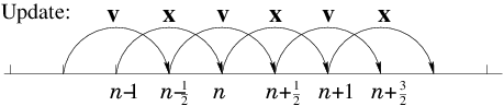
<?xml version="1.0"?>
<!DOCTYPE html    PUBLIC "-//W3C//DTD XHTML 1.1 plus MathML 2.0//EN"
           "http://www.w3.org/Math/DTD/mathml2/xhtml-math11-f.dtd">
<html xmlns="http://www.w3.org/1999/xhtml">
<head>
<meta name="GENERATOR" content="TtM 4.12" />
 <style type="text/css">
 div.p { margin-top: 7pt; }
 span.roman {font-family: serif; font-style: normal; font-weight: normal;} 
</style>
 <style type="text/css">
 .tiny {font-size:30%;}
 .scriptsize {font-size:xx-small;}
 .footnotesize {font-size:x-small;}
 .smaller {font-size:smaller;}
 .small {font-size:small;}
 .normalsize {font-size:medium;}
 .large {font-size:large;}
 .larger {font-size:x-large;}
 .largerstill {font-size:xx-large;}
 .huge {font-size:300%;}
 </style>
<title>chap2.xml</title>
</head>
<body><div>
<table width="100%"><tr><td>
 <a href="index.xml">HEAD</a></td><td align="right">
 <a href="chap1.xml">PREVIOUS
</a></td></tr></table>
 <a id="tth_chAp2"></a><h1>
Chapter 2 <br />Ordinary Differential Equations</h1>
<a id="ODEChap">
</a>

<div class="p"><!----></div>
<a 
id="ordinary_differential_equation2075"></a> <a id="tth_sEc2.1"></a><h2>
2.1&nbsp;&nbsp;Reduction to first-order</h2>

<div class="p"><!----></div>
<a 
id="reduction_of_order2176"></a><a 
id="order_reduction2177"></a> An ordinary
differential equation involves just one<a 
id="independent_variable2178"></a>
<em>independent</em> variable, <math xmlns="http://www.w3.org/1998/Math/MathML">
<mrow><mi>x</mi></mrow></math>, and a<a 
id="dependent_variable2179"></a>
<em>dependent</em> variable <math xmlns="http://www.w3.org/1998/Math/MathML">
<mrow><mi>y</mi></mrow></math>. Obviously it involves
<em>derivatives</em><a 
id="derivative2180"></a><a 
id="differential2181"></a> of the
dependent variable like <math xmlns="http://www.w3.org/1998/Math/MathML">
<mrow>
<mfrac><mrow><mi mathvariant="italic">dy</mi></mrow>
<mrow><mi mathvariant="italic">dx</mi></mrow>
</mfrac>
</mrow></math>. The highest
order<a 
id="order_of_differential2182"></a>
differential, i.e.&nbsp;the term <math xmlns="http://www.w3.org/1998/Math/MathML">
<mrow>
<mfrac><mrow>
<msup><mrow><mi>d</mi></mrow><mrow><mi>N</mi></mrow>
</msup>
<mi>y</mi></mrow>
<mrow>
<msup><mrow><mi mathvariant="italic">dx</mi></mrow><mrow><mi>N</mi></mrow>
</msup>
</mrow>
</mfrac>
</mrow></math> with the largest value
of <math xmlns="http://www.w3.org/1998/Math/MathML">
<mrow><mi>N</mi></mrow></math> appearing in the equation, defines the <em>order</em> <math xmlns="http://www.w3.org/1998/Math/MathML">
<mrow><mi>N</mi></mrow></math> of the
equation. So the most general ODE of order <math xmlns="http://www.w3.org/1998/Math/MathML">
<mrow><mi>N</mi></mrow></math> can be written such
that the <math xmlns="http://www.w3.org/1998/Math/MathML">
<mrow><mi>N</mi></mrow></math>th order derivative is equal to a function of all the
lower order derivatives and the independent variable <math xmlns="http://www.w3.org/1998/Math/MathML">
<mrow><mi>x</mi></mrow></math>:
<a id="ode1">
</a><br />
<table width="100%"><tr><td align="center">
    <math xmlns="http://www.w3.org/1998/Math/MathML">
    <mstyle displaystyle="true"><mrow>
<mfrac><mrow>
<msup><mrow><mi>d</mi></mrow><mrow><mi>N</mi></mrow>
</msup>
<mi>y</mi></mrow>
<mrow>
<msup><mrow><mi mathvariant="italic">dx</mi></mrow><mrow><mi>N</mi></mrow>
</msup>
</mrow>
</mfrac>
<mo>=</mo><mi>f</mi><mo stretchy="false">(</mo>
<mfrac><mrow>
<msup><mrow><mi>d</mi></mrow><mrow><mi>N</mi><mo>-</mo><mn>1</mn></mrow>
</msup>
<mi>y</mi></mrow>
<mrow>
<msup><mrow><mi mathvariant="italic">dx</mi></mrow><mrow><mi>N</mi><mo>-</mo><mn>1</mn></mrow>
</msup>
</mrow>
</mfrac>
<mo>,</mo>
<mfrac><mrow>
<msup><mrow><mi>d</mi></mrow><mrow><mi>N</mi><mo>-</mo><mn>2</mn></mrow>
</msup>
<mi>y</mi></mrow>
<mrow>
<msup><mrow><mi mathvariant="italic">dx</mi></mrow><mrow><mi>N</mi><mo>-</mo><mn>2</mn></mrow>
</msup>
</mrow>
</mfrac>
<mo>,</mo><mo>&#x2026;</mo><mo>,</mo>
<mfrac><mrow><mi mathvariant="italic">dy</mi></mrow>
<mrow><mi mathvariant="italic">dx</mi></mrow>
</mfrac>
<mo>,</mo><mi>y</mi><mo>,</mo><mi>x</mi><mo stretchy="false">)</mo></mrow>
    </mstyle></math></td><td width="1">
    <math xmlns="http://www.w3.org/1998/Math/MathML">
    <mstyle displaystyle="true"><mrow><mo stretchy="false">(</mo><mn>2</mn><mo>.</mo><mn>1</mn><mo stretchy="false">)</mo></mrow>
    </mstyle></math>
</td></tr></table>


<div class="p"><!----></div>
Such an ordinary differential equation of order <math xmlns="http://www.w3.org/1998/Math/MathML">
<mrow><mi>N</mi></mrow></math> in a single dependent
variable, <math xmlns="http://www.w3.org/1998/Math/MathML">
<mrow><mi>y</mi></mrow></math>, can always be reduced to a set of simultaneous
coupled<a 
id="coupled_equations2183"></a>
<em>first</em> order equations involving <math xmlns="http://www.w3.org/1998/Math/MathML">
<mrow><mi>N</mi></mrow></math> dependent variables. 
The simplest way to do this is to use a natural notation to denote by
<math xmlns="http://www.w3.org/1998/Math/MathML">
<mrow>
<msup><mrow><mi>y</mi></mrow><mrow><mo stretchy="false">(</mo><mi>i</mi><mo stretchy="false">)</mo></mrow>
</msup>
</mrow></math> the <math xmlns="http://www.w3.org/1998/Math/MathML">
<mrow><mi>i</mi></mrow></math>th derivative:
<a id="ode2">
</a><br />
<table width="100%"><tr><td align="center">
    <math xmlns="http://www.w3.org/1998/Math/MathML">
    <mstyle displaystyle="true"><mrow>
<mfrac><mrow>
<msup><mrow><mi>d</mi></mrow><mrow><mi>i</mi></mrow>
</msup>
<mi>y</mi></mrow>
<mrow>
<msup><mrow><mi mathvariant="italic">dx</mi></mrow><mrow><mi>i</mi></mrow>
</msup>
</mrow>
</mfrac>
<mo>=</mo>
<msup><mrow><mi>y</mi></mrow><mrow><mo stretchy="false">(</mo><mi>i</mi><mo stretchy="false">)</mo></mrow>
</msup>
<mi>&emsp;&emsp;&emsp;&emsp;&emsp;&emsp;</mi><mi>i</mi><mo>=</mo><mn>1</mn><mo>,</mo><mn>2</mn><mo>,</mo><mo>&#x2026;</mo><mo>,</mo><mi>N</mi><mo>-</mo><mn>1</mn><mo>.</mo></mrow>
    </mstyle></math></td><td width="1">
    <math xmlns="http://www.w3.org/1998/Math/MathML">
    <mstyle displaystyle="true"><mrow><mo stretchy="false">(</mo><mn>2</mn><mo>.</mo><mn>2</mn><mo stretchy="false">)</mo></mrow>
    </mstyle></math>
</td></tr></table>


When combined with the original equation, the total system can be
written as a first-order vector<a 
id="vector_equations2184"></a> differential
equation whose components are
<a id="ode3">
</a><br />
<table width="100%"><tr><td align="center">
    <math xmlns="http://www.w3.org/1998/Math/MathML">
    <mstyle displaystyle="true"><mrow>
<mfrac><mrow><mi>d</mi></mrow>
<mrow><mi mathvariant="italic">dx</mi></mrow>
</mfrac>

<msup><mrow><mi>y</mi></mrow><mrow><mo stretchy="false">(</mo><mi>i</mi><mo stretchy="false">)</mo></mrow>
</msup>
<mo>=</mo>
<msub><mrow><mi>f</mi></mrow><mrow><mi>i</mi></mrow>
</msub>
<mo stretchy="false">(</mo>
<msup><mrow><mi>y</mi></mrow><mrow><mo stretchy="false">(</mo><mi>N</mi><mo>-</mo><mn>1</mn><mo stretchy="false">)</mo></mrow>
</msup>
<mo>,</mo>
<msup><mrow><mi>y</mi></mrow><mrow><mo stretchy="false">(</mo><mi>N</mi><mo>-</mo><mn>2</mn><mo stretchy="false">)</mo></mrow>
</msup>
<mo>,</mo><mo>&#x2026;</mo><mo>,</mo>
<msup><mrow><mi>y</mi></mrow><mrow><mo stretchy="false">(</mo><mn>1</mn><mo stretchy="false">)</mo></mrow>
</msup>
<mo>,</mo>
<msup><mrow><mi>y</mi></mrow><mrow><mo stretchy="false">(</mo><mn>0</mn><mo stretchy="false">)</mo></mrow>
</msup>
<mo>,</mo><mi>x</mi><mo stretchy="false">)</mo><mo>,</mo><mi>&emsp;&emsp;&emsp;</mi><mi>i</mi><mo>=</mo><mn>0</mn><mo>,</mo><mn>1</mn><mo>,</mo><mo>&#x2026;</mo><mo>,</mo><mi>N</mi><mo>-</mo><mn>1</mn></mrow>
    </mstyle></math></td><td width="1">
    <math xmlns="http://www.w3.org/1998/Math/MathML">
    <mstyle displaystyle="true"><mrow><mo stretchy="false">(</mo><mn>2</mn><mo>.</mo><mn>3</mn><mo stretchy="false">)</mo></mrow>
    </mstyle></math>
</td></tr></table>


(where for notational consistency <math xmlns="http://www.w3.org/1998/Math/MathML">
<mrow>
<msup><mrow><mi>y</mi></mrow><mrow><mo stretchy="false">(</mo><mn>0</mn><mo stretchy="false">)</mo></mrow>
</msup>
<mo>=</mo><mi>y</mi></mrow></math>). Explicitly in vector form:
<a id="ode4">
</a><br />
<table width="100%"><tr><td align="center">
    <math xmlns="http://www.w3.org/1998/Math/MathML">
    <mstyle displaystyle="true"><mrow>
<mfrac><mrow><mi>d</mi></mrow>
<mrow><mi mathvariant="italic">dx</mi></mrow>
</mfrac>
<mrow><mo>(</mo>
<mtable>
<mtr><mtd columnalign="center"><mrow>
<msup><mrow><mi>y</mi></mrow><mrow><mo stretchy="false">(</mo><mn>0</mn><mo stretchy="false">)</mo></mrow>
</msup>
</mrow></mtd></mtr>
<mtr><mtd columnalign="center"><mrow>
<msup><mrow><mi>y</mi></mrow><mrow><mo stretchy="false">(</mo><mn>1</mn><mo stretchy="false">)</mo></mrow>
</msup>
</mrow></mtd></mtr>
<mtr><mtd columnalign="center"><mrow>:</mrow></mtd></mtr>
<mtr><mtd columnalign="center"><mrow>
<msup><mrow><mi>y</mi></mrow><mrow><mo stretchy="false">(</mo><mi>N</mi><mo>-</mo><mn>1</mn><mo stretchy="false">)</mo></mrow>
</msup>
</mrow></mtd></mtr></mtable>

<mo>)</mo></mrow><mo>=</mo><mrow><mo>(</mo>
<mtable>
<mtr><mtd columnalign="center"><mrow>
<msub><mrow><mi>f</mi></mrow><mrow><mn>0</mn></mrow>
</msub>
</mrow></mtd></mtr>
<mtr><mtd columnalign="center"><mrow>
<msub><mrow><mi>f</mi></mrow><mrow><mn>1</mn></mrow>
</msub>
</mrow></mtd></mtr>
<mtr><mtd columnalign="center"><mrow>:</mrow></mtd></mtr>
<mtr><mtd columnalign="center"><mrow>
<msub><mrow><mi>f</mi></mrow><mrow><mi>N</mi><mo>-</mo><mn>1</mn></mrow>
</msub>
</mrow></mtd></mtr></mtable>

<mo>)</mo></mrow><mo>=</mo><mrow><mo>(</mo>
<mtable>
<mtr><mtd columnalign="center"><mrow>
<msup><mrow><mi>y</mi></mrow><mrow><mo stretchy="false">(</mo><mn>1</mn><mo stretchy="false">)</mo></mrow>
</msup>
</mrow></mtd></mtr>
<mtr><mtd columnalign="center"><mrow>
<msup><mrow><mi>y</mi></mrow><mrow><mo stretchy="false">(</mo><mn>2</mn><mo stretchy="false">)</mo></mrow>
</msup>
</mrow></mtd></mtr>
<mtr><mtd columnalign="center"><mrow>:</mrow></mtd></mtr>
<mtr><mtd columnalign="center"><mrow><mi>f</mi><mo stretchy="false">(</mo>
<msup><mrow><mi>y</mi></mrow><mrow><mo stretchy="false">(</mo><mi>N</mi><mo>-</mo><mn>1</mn><mo stretchy="false">)</mo></mrow>
</msup>
<mo>,</mo>
<msup><mrow><mi>y</mi></mrow><mrow><mo stretchy="false">(</mo><mi>N</mi><mo>-</mo><mn>2</mn><mo stretchy="false">)</mo></mrow>
</msup>
<mo>,</mo><mo>&#x2026;</mo><mo>,</mo>
<msup><mrow><mi>y</mi></mrow><mrow><mo stretchy="false">(</mo><mn>1</mn><mo stretchy="false">)</mo></mrow>
</msup>
<mo>,</mo>
<msup><mrow><mi>y</mi></mrow><mrow><mo stretchy="false">(</mo><mn>0</mn><mo stretchy="false">)</mo></mrow>
</msup>
<mo>,</mo><mi>x</mi><mo stretchy="false">)</mo></mrow></mtd></mtr></mtable>

<mo>)</mo></mrow><mo>.</mo></mrow>
    </mstyle></math></td><td width="1">
    <math xmlns="http://www.w3.org/1998/Math/MathML">
    <mstyle displaystyle="true"><mrow><mo stretchy="false">(</mo><mn>2</mn><mo>.</mo><mn>4</mn><mo stretchy="false">)</mo></mrow>
    </mstyle></math>
</td></tr></table>


Recognizing that the combined simultanous vector system of dimension
<math xmlns="http://www.w3.org/1998/Math/MathML">
<mrow><mi>N</mi></mrow></math> with first-order derivatives, is equivalent to a single scalar equation
of order <math xmlns="http://www.w3.org/1998/Math/MathML">
<mrow><mi>N</mi></mrow></math>, we often say that the order<a 
id="order_of_system2185"></a> of the coupled vector system is
still <math xmlns="http://www.w3.org/1998/Math/MathML">
<mrow><mi>N</mi></mrow></math>. (Sorry if that seems confusing. In practice you get the
hang of it.)

<div class="p"><!----></div>
This is formal mathematics and applies to all equations, but precisely
such a set of coupled first-order equations will often also arise
directly in the formulation of the practical problem we are trying to
solve<a 
id="coupled_equations2186"></a>. Suppose
we are trying to track the position of a fluid<a 
id="fluid2187"></a> element in a three
dimensional steady flow<a 
id="flow2188"></a>. If we know the fluid velocity <math xmlns="http://www.w3.org/1998/Math/MathML">
<mrow><mi mathvariant="bold-italic">v</mi></mrow></math>
as a function of position <math xmlns="http://www.w3.org/1998/Math/MathML">
<mrow><mi mathvariant="bold-italic">v</mi><mo stretchy="false">(</mo><mi mathvariant="bold-italic">x</mi><mo stretchy="false">)</mo></mrow></math>, then the equation of the
track of a fluid element, i.e.&nbsp;the path followed by the element as it
moves in time <math xmlns="http://www.w3.org/1998/Math/MathML">
<mrow><mi>t</mi></mrow></math>, is
<a id="ode5">
</a><br />
<table width="100%"><tr><td align="center">
    <math xmlns="http://www.w3.org/1998/Math/MathML">
    <mstyle displaystyle="true"><mrow>
<mfrac><mrow><mi>d</mi></mrow>
<mrow><mi mathvariant="italic">dt</mi></mrow>
</mfrac>
<mi mathvariant="bold-italic">x</mi><mo>=</mo><mi mathvariant="bold-italic">v</mi><mo>.</mo></mrow>
    </mstyle></math></td><td width="1">
    <math xmlns="http://www.w3.org/1998/Math/MathML">
    <mstyle displaystyle="true"><mrow><mo stretchy="false">(</mo><mn>2</mn><mo>.</mo><mn>5</mn><mo stretchy="false">)</mo></mrow>
    </mstyle></math>
</td></tr></table>


This is the equation we must solve to find a fluid
streamline<a 
id="streamline2189"></a>.  It is of just the same form we derived
by order reduction. Such a history of position as a function of time
is called generically an orbit<a 
id="orbit2190"></a>.  Here the independent
variable is <math xmlns="http://www.w3.org/1998/Math/MathML">
<mrow><mi>t</mi></mrow></math>, and the dependent variable is <math xmlns="http://www.w3.org/1998/Math/MathML">
<mrow><mi mathvariant="bold-italic">x</mi></mrow></math>. The vector
<math xmlns="http://www.w3.org/1998/Math/MathML">
<mrow><mi mathvariant="bold-italic">v</mi></mrow></math> plays the role of the functions <math xmlns="http://www.w3.org/1998/Math/MathML">
<mrow>
<msub><mrow><mi>f</mi></mrow><mrow><mi>i</mi></mrow>
</msub>
</mrow></math>.

<div class="p"><!----></div>
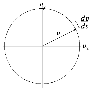
Orbits may not be just in space, they may be in
higher-dimensional<a 
id="higher-dimension2191"></a> phase-space. For example
(see Fig <a href="chap2.xml#cycvelocity">2.1</a>) to
find the orbit of a charged particle<a 
id="charged_particle2192"></a> (e.g.&nbsp;proton) of mass <math xmlns="http://www.w3.org/1998/Math/MathML">
<mrow>
<msub><mrow><mi>m</mi></mrow><mrow><mi>p</mi></mrow>
</msub>
</mrow></math> and charge <math xmlns="http://www.w3.org/1998/Math/MathML">
<mrow><mi>e</mi></mrow></math> moving at velocity <math xmlns="http://www.w3.org/1998/Math/MathML">
<mrow><mi mathvariant="bold-italic">v</mi></mrow></math> in a
uniform magnetic field <math xmlns="http://www.w3.org/1998/Math/MathML">
<mrow><mi mathvariant="bold-italic">B</mi></mrow></math><a 
id="magnetic_field2193"></a>, we observe
that it is subject to a force <math xmlns="http://www.w3.org/1998/Math/MathML">
<mrow><mi>e</mi><mi mathvariant="bold-italic">v</mi><mo>&times;</mo><mi mathvariant="bold-italic">B</mi></mrow></math>. In the absence
of any other forces, it has an equation of motion<a 
id="magnetic_force2194"></a>
<a id="ode6">
</a><br />
<table width="100%"><tr><td align="center">
    <math xmlns="http://www.w3.org/1998/Math/MathML">
    <mstyle displaystyle="true"><mrow>
<mfrac><mrow><mi>d</mi></mrow>
<mrow><mi mathvariant="italic">dt</mi></mrow>
</mfrac>
<mi mathvariant="bold-italic">v</mi><mo>=</mo>
<mfrac><mrow><mi>e</mi></mrow>
<mrow>
<msub><mrow><mi>m</mi></mrow><mrow><mi>p</mi></mrow>
</msub>
</mrow>
</mfrac>
<mi mathvariant="bold-italic">v</mi><mo>&times;</mo><mi mathvariant="bold-italic">B</mi><mo>=</mo><mi mathvariant="bold-italic">f</mi><mo stretchy="false">(</mo><mi mathvariant="bold-italic">v</mi><mo stretchy="false">)</mo><mo>,</mo></mrow>
    </mstyle></math></td><td width="1">
    <math xmlns="http://www.w3.org/1998/Math/MathML">
    <mstyle displaystyle="true"><mrow><mo stretchy="false">(</mo><mn>2</mn><mo>.</mo><mn>6</mn><mo stretchy="false">)</mo></mrow>
    </mstyle></math>
</td></tr></table>


in which the acceleration depends upon the velocity.  This is a first
order vector differential equation, in three dimensions, where <math xmlns="http://www.w3.org/1998/Math/MathML">
<mrow><mi>t</mi></mrow></math>
plays the role of the independent variable, and the dependent variable
is the vector velocity <math xmlns="http://www.w3.org/1998/Math/MathML">
<mrow><mi mathvariant="bold-italic">v</mi></mrow></math>. The vector
acceleration<a 
id="acceleration2195"></a> <math xmlns="http://www.w3.org/1998/Math/MathML">
<mrow><mi mathvariant="bold-italic">f</mi></mrow></math> which is the vector
derivative function depends upon all the components of <math xmlns="http://www.w3.org/1998/Math/MathML">
<mrow><mi mathvariant="bold-italic">v</mi></mrow></math>.

<div class="p"><!----></div>
<a id="tth_fIg2.1">
</a>   <img src="figures/cycvelocity.png" alt="figures/cycvelocity.png" /><a id="cycvelocity">
</a>
  
<div style="text-align:center">Figure 2.1: Orbit of the velocity of a particle moving in a uniform
    magnetic field is a circle in <em>velocity-space</em> perpendicular
    to the field (<math xmlns="http://www.w3.org/1998/Math/MathML">
<mrow><mi>B</mi><mo>=</mo><mi>B</mi>
<mover><mrow><mi mathvariant="bold-italic">z</mi></mrow>
<mo>&Hat;</mo></mover>
</mrow></math> here).<a id="cycvelocity">
</a></div>

<div class="p"><!----></div>
If, for our proton orbit, <math xmlns="http://www.w3.org/1998/Math/MathML">
<mrow><mi mathvariant="bold-italic">B</mi></mrow></math> is not uniform, but varies with
position, then we need to know both position <math xmlns="http://www.w3.org/1998/Math/MathML">
<mrow><mi mathvariant="bold-italic">x</mi></mrow></math>, and velocity
<math xmlns="http://www.w3.org/1998/Math/MathML">
<mrow><mi mathvariant="bold-italic">v</mi></mrow></math> at all times along the orbit to solve it. The system then
involves six-dimensional vectors consisting of the components of
<math xmlns="http://www.w3.org/1998/Math/MathML">
<mrow><mi mathvariant="bold-italic">x</mi></mrow></math> and <math xmlns="http://www.w3.org/1998/Math/MathML">
<mrow><mi mathvariant="bold-italic">v</mi></mrow></math>:

<div class="p"><!----></div>
<a id="ode7">
</a><br />
<table width="100%"><tr><td align="center">
    <math xmlns="http://www.w3.org/1998/Math/MathML">
    <mstyle displaystyle="true"><mrow>
<mfrac><mrow><mi>d</mi></mrow>
<mrow><mi mathvariant="italic">dt</mi></mrow>
</mfrac>
<mrow><mo>(</mo>
<mtable>
<mtr><mtd columnalign="center"><mrow>
<msub><mrow><mi>x</mi></mrow><mrow><mn>1</mn></mrow>
</msub>
</mrow></mtd></mtr>
<mtr><mtd columnalign="center"><mrow>
<msub><mrow><mi>x</mi></mrow><mrow><mn>2</mn></mrow>
</msub>
</mrow></mtd></mtr>
<mtr><mtd columnalign="center"><mrow>
<msub><mrow><mi>x</mi></mrow><mrow><mn>3</mn></mrow>
</msub>
</mrow></mtd></mtr>
<mtr><mtd columnalign="center"><mrow>
<msub><mrow><mi>v</mi></mrow><mrow><mn>1</mn></mrow>
</msub>
</mrow></mtd></mtr>
<mtr><mtd columnalign="center"><mrow>
<msub><mrow><mi>v</mi></mrow><mrow><mn>2</mn></mrow>
</msub>
</mrow></mtd></mtr>
<mtr><mtd columnalign="center"><mrow>
<msub><mrow><mi>v</mi></mrow><mrow><mn>3</mn></mrow>
</msub>
</mrow></mtd></mtr></mtable>

<mo>)</mo></mrow><mo>=</mo><mrow><mo>(</mo>
<mtable>
<mtr><mtd columnalign="center"><mrow>
<msub><mrow><mi>v</mi></mrow><mrow><mn>1</mn></mrow>
</msub>
</mrow></mtd></mtr>
<mtr><mtd columnalign="center"><mrow>
<msub><mrow><mi>v</mi></mrow><mrow><mn>2</mn></mrow>
</msub>
</mrow></mtd></mtr>
<mtr><mtd columnalign="center"><mrow>
<msub><mrow><mi>v</mi></mrow><mrow><mn>3</mn></mrow>
</msub>
</mrow></mtd></mtr>
<mtr><mtd columnalign="center"><mrow><mo stretchy="false">(</mo>
<msub><mrow><mi>v</mi></mrow><mrow><mn>2</mn></mrow>
</msub>

<msub><mrow><mi>B</mi></mrow><mrow><mn>3</mn></mrow>
</msub>
<mo>-</mo>
<msub><mrow><mi>v</mi></mrow><mrow><mn>3</mn></mrow>
</msub>

<msub><mrow><mi>B</mi></mrow><mrow><mn>2</mn></mrow>
</msub>
<mo stretchy="false">)</mo><mi>e</mi><mo stretchy="false">/</mo>
<msub><mrow><mi>m</mi></mrow><mrow><mi>p</mi></mrow>
</msub>
</mrow></mtd></mtr>
<mtr><mtd columnalign="center"><mrow><mo stretchy="false">(</mo>
<msub><mrow><mi>v</mi></mrow><mrow><mn>3</mn></mrow>
</msub>

<msub><mrow><mi>B</mi></mrow><mrow><mn>1</mn></mrow>
</msub>
<mo>-</mo>
<msub><mrow><mi>v</mi></mrow><mrow><mn>1</mn></mrow>
</msub>

<msub><mrow><mi>B</mi></mrow><mrow><mn>3</mn></mrow>
</msub>
<mo stretchy="false">)</mo><mi>e</mi><mo stretchy="false">/</mo>
<msub><mrow><mi>m</mi></mrow><mrow><mi>p</mi></mrow>
</msub>
</mrow></mtd></mtr>
<mtr><mtd columnalign="center"><mrow><mo stretchy="false">(</mo>
<msub><mrow><mi>v</mi></mrow><mrow><mn>1</mn></mrow>
</msub>

<msub><mrow><mi>B</mi></mrow><mrow><mn>2</mn></mrow>
</msub>
<mo>-</mo>
<msub><mrow><mi>v</mi></mrow><mrow><mn>2</mn></mrow>
</msub>

<msub><mrow><mi>B</mi></mrow><mrow><mn>1</mn></mrow>
</msub>
<mo stretchy="false">)</mo><mi>e</mi><mo stretchy="false">/</mo>
<msub><mrow><mi>m</mi></mrow><mrow><mi>p</mi></mrow>
</msub>
</mrow></mtd></mtr></mtable>

<mo>)</mo></mrow><mo>.</mo></mrow>
    </mstyle></math></td><td width="1">
    <math xmlns="http://www.w3.org/1998/Math/MathML">
    <mstyle displaystyle="true"><mrow><mo stretchy="false">(</mo><mn>2</mn><mo>.</mo><mn>7</mn><mo stretchy="false">)</mo></mrow>
    </mstyle></math>
</td></tr></table>


<div class="p"><!----></div>
Very often, to find <em>analytic</em> solutions it feels more natural to
eliminate some of the dependent variables with the result that the
order of the ODE is raised. So, for example for a uniform magnetic
field in the <math xmlns="http://www.w3.org/1998/Math/MathML">
<mrow><mn>3</mn></mrow></math>-direction, the dynamics perpendicular to it separate
out into
<a id="ode8">
</a><br />
<table width="100%"><tr><td align="center">
    <math xmlns="http://www.w3.org/1998/Math/MathML">
    <mstyle displaystyle="true"><mrow>
<mfrac><mrow><mi>d</mi></mrow>
<mrow><mi mathvariant="italic">dt</mi></mrow>
</mfrac>

<msub><mrow><mi>v</mi></mrow><mrow><mn>1</mn></mrow>
</msub>
<mo>=</mo><mi mathvariant="italic">&Omega;</mi>
<msub><mrow><mi>v</mi></mrow><mrow><mn>2</mn></mrow>
</msub>
<mo>,</mo><mi>&ensp;</mi>
<mfrac><mrow><mi>d</mi></mrow>
<mrow><mi mathvariant="italic">dt</mi></mrow>
</mfrac>

<msub><mrow><mi>v</mi></mrow><mrow><mn>2</mn></mrow>
</msub>
<mo>=</mo><mo>-</mo><mi mathvariant="italic">&Omega;</mi>
<msub><mrow><mi>v</mi></mrow><mrow><mn>1</mn></mrow>
</msub>
<mi>&emsp;&emsp;&emsp;</mi><mo>&rArr;</mo><mi>&emsp;&emsp;&emsp;</mi>
<mfrac><mrow>
<msup><mrow><mi>d</mi></mrow><mrow><mn>2</mn></mrow>
</msup>

<msub><mrow><mi>v</mi></mrow><mrow><mn>1</mn></mrow>
</msub>
</mrow>
<mrow>
<msup><mrow><mi mathvariant="italic">dt</mi></mrow><mrow><mn>2</mn></mrow>
</msup>
</mrow>
</mfrac>
<mo>=</mo><mo>-</mo>
<msup><mrow><mi mathvariant="italic">&Omega;</mi></mrow><mrow><mn>2</mn></mrow>
</msup>

<msub><mrow><mi>v</mi></mrow><mrow><mn>1</mn></mrow>
</msub>
<mo>,</mo><mi>&ensp;</mi>
<mfrac><mrow>
<msup><mrow><mi>d</mi></mrow><mrow><mn>2</mn></mrow>
</msup>

<msub><mrow><mi>v</mi></mrow><mrow><mn>2</mn></mrow>
</msub>
</mrow>
<mrow>
<msup><mrow><mi mathvariant="italic">dt</mi></mrow><mrow><mn>2</mn></mrow>
</msup>
</mrow>
</mfrac>
<mo>=</mo><mo>-</mo>
<msup><mrow><mi mathvariant="italic">&Omega;</mi></mrow><mrow><mn>2</mn></mrow>
</msup>

<msub><mrow><mi>v</mi></mrow><mrow><mn>2</mn></mrow>
</msub>
<mo>.</mo></mrow>
    </mstyle></math></td><td width="1">
    <math xmlns="http://www.w3.org/1998/Math/MathML">
    <mstyle displaystyle="true"><mrow><mo stretchy="false">(</mo><mn>2</mn><mo>.</mo><mn>8</mn><mo stretchy="false">)</mo></mrow>
    </mstyle></math>
</td></tr></table>


(writing <math xmlns="http://www.w3.org/1998/Math/MathML">
<mrow><mi mathvariant="italic">&Omega;</mi><mo>=</mo><mi mathvariant="italic">eB</mi><mo stretchy="false">/</mo>
<msub><mrow><mi>m</mi></mrow><mrow><mi>p</mi></mrow>
</msub>
</mrow></math>)<a 
id="cyclotron_frequency___Omega_2196"></a>.  The second-order
<em>uncoupled</em> equations are familiar to us as simple harmonic
oscillator<a 
id="simple_harmonic_oscillator2197"></a> equations, having
solutions like <math xmlns="http://www.w3.org/1998/Math/MathML">
<mrow><mi>cos</mi><mi mathvariant="italic">&Omega;</mi><mi>t</mi></mrow></math> and <math xmlns="http://www.w3.org/1998/Math/MathML">
<mrow><mi>sin</mi><mi mathvariant="italic">&Omega;</mi><mi>t</mi></mrow></math>. So they are easier
to solve <em>analytically</em>. But the original first-order equations,
even though they are <em>coupled</em> are far easier to solve
<em>numerically</em>. So we don't generally do the
elimination<a 
id="elimination2198"></a> in computational solutions.

<div class="p"><!----></div>
 <a id="tth_sEc2.2"></a><h2>
2.2&nbsp;&nbsp;Numerical Integration of Initial Value Problem</h2>

<div class="p"><!----></div>
     <a id="tth_sEc2.2.1"></a><h3>
2.2.1&nbsp;&nbsp;Explicit Integration</h3>
Now we consider how in practice to solve a first-order ODE<a 
id="ODE2299"></a>
in which all the boundary conditions<a 
id="boundary_condition22100"></a> are
imposed at the same position in the independent variable. Such
boundary conditions constitute what is called an "initial value
problem"<a 
id="initial_value_problem22101"></a>. We start
integrating<a 
id="integrating22102"></a> forward in the independent variable
(e.g. time or space) from a place where the initial values are
specified. To simplify the discussion we will consider a single
(scalar) dependent variable <math xmlns="http://www.w3.org/1998/Math/MathML">
<mrow><mi>y</mi></mrow></math>, but note that the generalization to a
vector of dependent variables is usually immediate, so the treatment
is fine for higher order equations that have been reduced to vectorial
first-order form.

<div class="p"><!----></div>
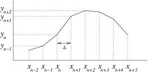
In general, numerical solution of differential equations requires us
to represent the solution, which is usually continuous, in a
discrete<a 
id="discrete_representation22103"></a>
manner where the values are given at a series of points rather than
continuously. See Fig.&nbsp;<a href="chap2.xml#discretegradientl">2.2</a>.

<div class="p"><!----></div>
<a id="tth_fIg2.2">
</a>   <img src="figures/discretegradient.png" alt="figures/discretegradient.png" /><a id="discretegradient">
</a>
  
<div style="text-align:center">Figure 2.2: Illustrating finite difference representation of a
    continuous function.</div>
  <a id="discretegradientl">
</a>

<div class="p"><!----></div>
The natural way to discretize the
derivative<a 
id="discrete_derivative22104"></a> is to write
<a id="ode9">
</a><br />
<table width="100%"><tr><td align="center">
    <math xmlns="http://www.w3.org/1998/Math/MathML">
    <mstyle displaystyle="true"><mrow>
<mfrac><mrow><mi mathvariant="italic">dy</mi></mrow>
<mrow><mi mathvariant="italic">dx</mi></mrow>
</mfrac>
<mo>&ap;</mo>
<mfrac><mrow>
<msub><mrow><mi>y</mi></mrow><mrow><mi>n</mi><mo>+</mo><mn>1</mn></mrow>
</msub>
<mo>-</mo>
<msub><mrow><mi>y</mi></mrow><mrow><mi>n</mi></mrow>
</msub>
</mrow>
<mrow>
<msub><mrow><mi>x</mi></mrow><mrow><mi>n</mi><mo>+</mo><mn>1</mn></mrow>
</msub>
<mo>-</mo>
<msub><mrow><mi>x</mi></mrow><mrow><mi>n</mi></mrow>
</msub>
</mrow>
</mfrac>
<mo>=</mo><mi>f</mi><mo stretchy="false">(</mo><mi>y</mi><mo>,</mo><mi>x</mi><mo stretchy="false">)</mo><mo>,</mo></mrow>
    </mstyle></math></td><td width="1">
    <math xmlns="http://www.w3.org/1998/Math/MathML">
    <mstyle displaystyle="true"><mrow><mo stretchy="false">(</mo><mn>2</mn><mo>.</mo><mn>9</mn><mo stretchy="false">)</mo></mrow>
    </mstyle></math>
</td></tr></table>


where the index<a 
id="index22105"></a> <math xmlns="http://www.w3.org/1998/Math/MathML">
<mrow><mi>n</mi></mrow></math> denotes the value at the <math xmlns="http://www.w3.org/1998/Math/MathML">
<mrow><mi>n</mi></mrow></math>th
discrete step, and therefore
<a id="ode10">
</a><br />
<table width="100%"><tr><td align="center">
    <math xmlns="http://www.w3.org/1998/Math/MathML">
    <mstyle displaystyle="true"><mrow>
<msub><mrow><mi>y</mi></mrow><mrow><mi>n</mi><mo>+</mo><mn>1</mn></mrow>
</msub>
<mo>=</mo>
<msub><mrow><mi>y</mi></mrow><mrow><mi>n</mi></mrow>
</msub>
<mo>+</mo><mi>f</mi><mo stretchy="false">(</mo><mi>y</mi><mo>,</mo><mi>x</mi><mo stretchy="false">)</mo><mo stretchy="false">(</mo>
<msub><mrow><mi>x</mi></mrow><mrow><mi>n</mi><mo>+</mo><mn>1</mn></mrow>
</msub>
<mo>-</mo>
<msub><mrow><mi>x</mi></mrow><mrow><mi>n</mi></mrow>
</msub>
<mo stretchy="false">)</mo><mo>.</mo></mrow>
    </mstyle></math></td><td width="1">
    <math xmlns="http://www.w3.org/1998/Math/MathML">
    <mstyle displaystyle="true"><mrow><mo stretchy="false">(</mo><mn>2</mn><mo>.</mo><mn>10</mn><mo stretchy="false">)</mo></mrow>
    </mstyle></math>
</td></tr></table>


This equation tells us how <math xmlns="http://www.w3.org/1998/Math/MathML">
<mrow><mi>y</mi></mrow></math> changes from one step to the
next. Starting from an initial position we can step discretely as far
as we like, choosing the size of the independent variable step
<math xmlns="http://www.w3.org/1998/Math/MathML">
<mrow><mo stretchy="false">(</mo>
<msub><mrow><mi>x</mi></mrow><mrow><mi>n</mi><mo>+</mo><mn>1</mn></mrow>
</msub>
<mo>-</mo>
<msub><mrow><mi>x</mi></mrow><mrow><mi>n</mi></mrow>
</msub>
<mo stretchy="false">)</mo><mo>=</mo><mi mathvariant="italic">&Delta;</mi></mrow></math> appropriately. 

<div class="p"><!----></div>
A question that arises, though, is what to use for <math xmlns="http://www.w3.org/1998/Math/MathML">
<mrow><mi>x</mi></mrow></math> and <math xmlns="http://www.w3.org/1998/Math/MathML">
<mrow><mi>y</mi></mrow></math> inside
the derivative function <math xmlns="http://www.w3.org/1998/Math/MathML">
<mrow><mi>f</mi><mo stretchy="false">(</mo><mi>y</mi><mo>,</mo><mi>x</mi><mo stretchy="false">)</mo></mrow></math>. The <math xmlns="http://www.w3.org/1998/Math/MathML">
<mrow><mi>x</mi></mrow></math> value can be chosen more or
less at will<a href="footnote.xml#tthFtNtABD" id="tthFrefABD"><math xmlns="http://www.w3.org/1998/Math/MathML">
<mrow>
<msup><mrow></mrow><mrow><mn>13</mn></mrow>
</msup>
</mrow></math></a>
but before we've actually made the step, we don't know where we are
going to end up in <math xmlns="http://www.w3.org/1998/Math/MathML">
<mrow><mi>y</mi></mrow></math>, so we can't easily decide where in <math xmlns="http://www.w3.org/1998/Math/MathML">
<mrow><mi>y</mi></mrow></math> to
evaluate <math xmlns="http://www.w3.org/1998/Math/MathML">
<mrow><mi>f</mi></mrow></math>. The easiest answer, but not generally the best, is to
recognize that at any point in stepping from <math xmlns="http://www.w3.org/1998/Math/MathML">
<mrow><mi>n</mi></mrow></math> to <math xmlns="http://www.w3.org/1998/Math/MathML">
<mrow><mi>n</mi><mo>+</mo><mn>1</mn></mrow></math> along the
orbit, we already have the value <math xmlns="http://www.w3.org/1998/Math/MathML">
<mrow>
<msub><mrow><mi>y</mi></mrow><mrow><mi>n</mi></mrow>
</msub>
</mrow></math>. So we could just use
<math xmlns="http://www.w3.org/1998/Math/MathML">
<mrow><mi>f</mi><mo stretchy="false">(</mo>
<msub><mrow><mi>y</mi></mrow><mrow><mi>n</mi></mrow>
</msub>
<mo>,</mo>
<msub><mrow><mi>x</mi></mrow><mrow><mi>n</mi></mrow>
</msub>
<mo stretchy="false">)</mo></mrow></math>. This choice is said to be
"explicit"<a 
id="explicit_method22106"></a>, and is sometimes called the Euler
method<a 
id="Euler_method22107"></a>. The reason why this method is not the best
is because it tends have poor <em>accuracy</em><a 
id="accuracy22108"></a> and poor
<em>stability</em><a 
id="stability22109"></a>.

<div class="p"><!----></div>
     <a id="tth_sEc2.2.2"></a><h3>
2.2.2&nbsp;&nbsp;Accuracy and Runge-Kutta Schemes</h3>

<div class="p"><!----></div>
<a 
id="Runge-Kutta_schemes22110"></a> To illustrate the problem of accuracy, consider
the derivative function <math xmlns="http://www.w3.org/1998/Math/MathML">
<mrow><mi>f</mi></mrow></math> expanded as a 
Taylor<a 
id="Taylor_expansion22111"></a> series about the <math xmlns="http://www.w3.org/1998/Math/MathML">
<mrow>
<msub><mrow><mi>x</mi></mrow><mrow><mi>n</mi></mrow>
</msub>
<mo>,</mo>
<msub><mrow><mi>y</mi></mrow><mrow><mi>n</mi></mrow>
</msub>
</mrow></math> position, writing
<math xmlns="http://www.w3.org/1998/Math/MathML">
<mrow><mi>x</mi><mo>-</mo>
<msub><mrow><mi>x</mi></mrow><mrow><mi>n</mi></mrow>
</msub>
<mo>=</mo><mi mathvariant="italic">&delta;</mi><mi>x</mi></mrow></math>, <math xmlns="http://www.w3.org/1998/Math/MathML">
<mrow><mi>y</mi><mo>-</mo>
<msub><mrow><mi>y</mi></mrow><mrow><mi>n</mi></mrow>
</msub>
<mo>=</mo><mi mathvariant="italic">&delta;</mi><mi>y</mi></mrow></math>. The derivative function <math xmlns="http://www.w3.org/1998/Math/MathML">
<mrow><mi>f</mi></mrow></math> is a
function of both <math xmlns="http://www.w3.org/1998/Math/MathML">
<mrow><mi>x</mi></mrow></math> and <math xmlns="http://www.w3.org/1998/Math/MathML">
<mrow><mi>y</mi></mrow></math>. However, the solution for the orbit can
be written <math xmlns="http://www.w3.org/1998/Math/MathML">
<mrow><mi>y</mi><mo>=</mo><mi>y</mi><mo stretchy="false">(</mo><mi>x</mi><mo stretchy="false">)</mo></mrow></math>. Therefore the function evaluated on the orbit,
<math xmlns="http://www.w3.org/1998/Math/MathML">
<mrow><mi>f</mi><mo stretchy="false">(</mo><mi>y</mi><mo stretchy="false">(</mo><mi>x</mi><mo stretchy="false">)</mo><mo>,</mo><mi>x</mi><mo stretchy="false">)</mo></mrow></math>, is a function only of <math xmlns="http://www.w3.org/1998/Math/MathML">
<mrow><mi>x</mi></mrow></math>, and we can write its (total)
derivative as <math xmlns="http://www.w3.org/1998/Math/MathML">
<mrow>
<mfrac><mrow><mi mathvariant="italic">df</mi></mrow>
<mrow><mi mathvariant="italic">dx</mi></mrow>
</mfrac>
</mrow></math>.
The Taylor expansion of this function is simply<a href="footnote.xml#tthFtNtABE" id="tthFrefABE"><math xmlns="http://www.w3.org/1998/Math/MathML">
<mrow>
<msup><mrow></mrow><mrow><mn>14</mn></mrow>
</msup>
</mrow></math></a>
<a id="ode12">
</a><br />
<table width="100%"><tr><td align="center">
    <math xmlns="http://www.w3.org/1998/Math/MathML">
    <mstyle displaystyle="true"><mrow><mi>f</mi><mo stretchy="false">(</mo><mi>y</mi><mo stretchy="false">(</mo><mi>x</mi><mo stretchy="false">)</mo><mo>,</mo><mi>x</mi><mo stretchy="false">)</mo><mo>=</mo><mi>f</mi><mo stretchy="false">(</mo>
<msub><mrow><mi>y</mi></mrow><mrow><mi>n</mi></mrow>
</msub>
<mo>,</mo>
<msub><mrow><mi>x</mi></mrow><mrow><mi>n</mi></mrow>
</msub>
<mo stretchy="false">)</mo><mo>+</mo>
<mfrac><mrow>
<msub><mrow><mi mathvariant="italic">df</mi></mrow><mrow><mi>n</mi></mrow>
</msub>
</mrow>
<mrow><mi mathvariant="italic">dx</mi></mrow>
</mfrac>
<mi mathvariant="italic">&delta;</mi><mi>x</mi><mo>+</mo>
<mfrac><mrow>
<msup><mrow><mi>d</mi></mrow><mrow><mn>2</mn></mrow>
</msup>

<msub><mrow><mi>f</mi></mrow><mrow><mi>n</mi></mrow>
</msub>
</mrow>
<mrow>
<msup><mrow><mi mathvariant="italic">dx</mi></mrow><mrow><mn>2</mn></mrow>
</msup>
</mrow>
</mfrac>

<mfrac><mrow><mi mathvariant="italic">&delta;</mi>
<msup><mrow><mi>x</mi></mrow><mrow><mn>2</mn></mrow>
</msup>
</mrow>
<mrow><mn>2</mn><mo>!</mo></mrow>
</mfrac>
<mo>+</mo><mi>O</mi><mo stretchy="false">(</mo><mi mathvariant="italic">&delta;</mi>
<msup><mrow><mi>x</mi></mrow><mrow><mn>3</mn></mrow>
</msup>
<mo stretchy="false">)</mo></mrow>
    </mstyle></math></td><td width="1">
    <math xmlns="http://www.w3.org/1998/Math/MathML">
    <mstyle displaystyle="true"><mrow><mo stretchy="false">(</mo><mn>2</mn><mo>.</mo><mn>11</mn><mo stretchy="false">)</mo></mrow>
    </mstyle></math>
</td></tr></table>


We use the notation <math xmlns="http://www.w3.org/1998/Math/MathML">
<mrow>
<msub><mrow><mi mathvariant="italic">df</mi></mrow><mrow><mi>n</mi></mrow>
</msub>
<mo stretchy="false">/</mo><mi mathvariant="italic">dx</mi></mrow></math> (etc.) to indicate values evaluated at
position <math xmlns="http://www.w3.org/1998/Math/MathML">
<mrow><mi>n</mi></mrow></math>.
If we substitute this Taylor expansion for <math xmlns="http://www.w3.org/1998/Math/MathML">
<mrow><mi>f</mi></mrow></math> into the differential
equation we are trying to solve,
 <math xmlns="http://www.w3.org/1998/Math/MathML">
<mrow><mi mathvariant="italic">dy</mi><mo stretchy="false">/</mo><mi mathvariant="italic">dx</mi><mo>=</mo><mi>d</mi><mi mathvariant="italic">&delta;</mi><mi>y</mi><mo stretchy="false">/</mo><mi>d</mi><mi mathvariant="italic">&delta;</mi><mi>x</mi><mo>=</mo><mi>f</mi></mrow></math>,
and integrate term by term we
get the <em>exact</em> solution of the differential equation.
<a id="ode13">
</a><br />
<table width="100%"><tr><td align="center">
    <math xmlns="http://www.w3.org/1998/Math/MathML">
    <mstyle displaystyle="true"><mrow><mi mathvariant="italic">&delta;</mi><mi>y</mi><mo>=</mo>
<msub><mrow><mi>f</mi></mrow><mrow><mi>n</mi></mrow>
</msub>
<mi mathvariant="italic">&delta;</mi><mi>x</mi><mo>+</mo>
<mfrac><mrow>
<msub><mrow><mi mathvariant="italic">df</mi></mrow><mrow><mi>n</mi></mrow>
</msub>
</mrow>
<mrow><mi mathvariant="italic">dx</mi></mrow>
</mfrac>

<mfrac><mrow><mi mathvariant="italic">&delta;</mi>
<msup><mrow><mi>x</mi></mrow><mrow><mn>2</mn></mrow>
</msup>
</mrow>
<mrow><mn>2</mn><mo>!</mo></mrow>
</mfrac>
<mo>+</mo>
<mfrac><mrow>
<msup><mrow><mi>d</mi></mrow><mrow><mn>2</mn></mrow>
</msup>

<msub><mrow><mi>f</mi></mrow><mrow><mi>n</mi></mrow>
</msub>
</mrow>
<mrow>
<msup><mrow><mi mathvariant="italic">dx</mi></mrow><mrow><mn>2</mn></mrow>
</msup>
</mrow>
</mfrac>

<mfrac><mrow><mi mathvariant="italic">&delta;</mi>
<msup><mrow><mi>x</mi></mrow><mrow><mn>3</mn></mrow>
</msup>
</mrow>
<mrow><mn>3</mn><mo>!</mo></mrow>
</mfrac>
<mo>+</mo><mi>O</mi><mo stretchy="false">(</mo><mi mathvariant="italic">&delta;</mi>
<msup><mrow><mi>x</mi></mrow><mrow><mn>4</mn></mrow>
</msup>
<mo stretchy="false">)</mo></mrow>
    </mstyle></math></td><td width="1">
    <math xmlns="http://www.w3.org/1998/Math/MathML">
    <mstyle displaystyle="true"><mrow><mo stretchy="false">(</mo><mn>2</mn><mo>.</mo><mn>12</mn><mo stretchy="false">)</mo></mrow>
    </mstyle></math>
</td></tr></table>


We subtract from it whatever the finite difference <em>approximate</em>
equation is. In the case of
(<a href="chap2.xml#ode10">2.10</a>) it is <math xmlns="http://www.w3.org/1998/Math/MathML">
<mrow><mi mathvariant="italic">&delta;</mi>
<msup><mrow><mi>y</mi></mrow><mrow><mo stretchy="false">(</mo><mn>1</mn><mo stretchy="false">)</mo></mrow>
</msup>
<mo>=</mo>
<msub><mrow><mi>f</mi></mrow><mrow><mi>n</mi></mrow>
</msub>
<mi mathvariant="italic">&delta;</mi><mi>x</mi></mrow></math>, and we find that the error<a 
id="error_Runge-Kutta22112"></a> in
<math xmlns="http://www.w3.org/1998/Math/MathML">
<mrow>
<msub><mrow><mi>y</mi></mrow><mrow><mi>n</mi><mo>+</mo><mn>1</mn></mrow>
</msub>
</mrow></math> is 
<a id="ode14">
</a><br />
<table width="100%"><tr><td align="center">
    <math xmlns="http://www.w3.org/1998/Math/MathML">
    <mstyle displaystyle="true"><mrow><mi mathvariant="italic">&delta;</mi><mi>y</mi><mo>-</mo><mi mathvariant="italic">&delta;</mi>
<msup><mrow><mi>y</mi></mrow><mrow><mo stretchy="false">(</mo><mn>1</mn><mo stretchy="false">)</mo></mrow>
</msup>
<mo>=</mo><mi mathvariant="italic">&epsi;</mi><mo>=</mo>
<mfrac><mrow>
<msub><mrow><mi mathvariant="italic">df</mi></mrow><mrow><mi>n</mi></mrow>
</msub>
</mrow>
<mrow><mi mathvariant="italic">dx</mi></mrow>
</mfrac>

<mfrac><mrow><mi mathvariant="italic">&delta;</mi>
<msup><mrow><mi>x</mi></mrow><mrow><mn>2</mn></mrow>
</msup>
</mrow>
<mrow><mn>2</mn><mo>!</mo></mrow>
</mfrac>
<mo>+</mo>
<mfrac><mrow>
<msup><mrow><mi>d</mi></mrow><mrow><mn>2</mn></mrow>
</msup>

<msub><mrow><mi>f</mi></mrow><mrow><mi>n</mi></mrow>
</msub>
</mrow>
<mrow>
<msup><mrow><mi mathvariant="italic">dx</mi></mrow><mrow><mn>2</mn></mrow>
</msup>
</mrow>
</mfrac>

<mfrac><mrow><mi mathvariant="italic">&delta;</mi>
<msup><mrow><mi>x</mi></mrow><mrow><mn>3</mn></mrow>
</msup>
</mrow>
<mrow><mn>3</mn><mo>!</mo></mrow>
</mfrac>
<mo>+</mo><mi>O</mi><mo stretchy="false">(</mo><mi mathvariant="italic">&delta;</mi>
<msup><mrow><mi>x</mi></mrow><mrow><mn>4</mn></mrow>
</msup>
<mo stretchy="false">)</mo><mo>.</mo></mrow>
    </mstyle></math></td><td width="1">
    <math xmlns="http://www.w3.org/1998/Math/MathML">
    <mstyle displaystyle="true"><mrow><mo stretchy="false">(</mo><mn>2</mn><mo>.</mo><mn>13</mn><mo stretchy="false">)</mo></mrow>
    </mstyle></math>
</td></tr></table>


This tells us that the explicit Euler difference scheme is accurate
only to <em>first-order</em><a 
id="error_order22113"></a><a 
id="order_of___error22114"></a><a 
id="first-order22115"></a> in
the size of the step <math xmlns="http://www.w3.org/1998/Math/MathML">
<mrow><mi mathvariant="italic">&delta;</mi><mi>x</mi></mrow></math> (when the first derivative of <math xmlns="http://www.w3.org/1998/Math/MathML">
<mrow><mi>f</mi></mrow></math> is
non-zero) because an error of order <math xmlns="http://www.w3.org/1998/Math/MathML">
<mrow><mi mathvariant="italic">&delta;</mi>
<msup><mrow><mi>x</mi></mrow><mrow><mn>2</mn></mrow>
</msup>
</mrow></math> is present.  That
means if we make the step a factor of 2 smaller, the cumulative error,
when integrating over a set total distance, gets smaller by
(approximately) a factor of 2. (Because each step's error is 4 times
smaller, but there are twice as many steps.) That's not very good. We
would have to take very small steps, <math xmlns="http://www.w3.org/1998/Math/MathML">
<mrow><mi mathvariant="italic">&delta;</mi><mi>x</mi></mrow></math>, to get good accuracy.

<div class="p"><!----></div>
<a id="tth_fIg2.3">
</a>   <img src="figures/fnplus1.png" alt="figures/fnplus1.png" /><a id="fnplus1">
</a>
  
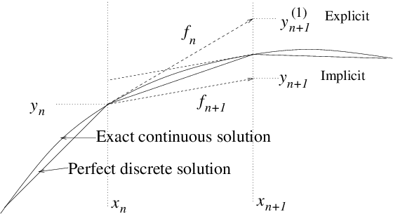
<div style="text-align:center">Figure 2.3: Optional steps using derivative function evaluated at <math xmlns="http://www.w3.org/1998/Math/MathML">
<mrow><mi>n</mi></mrow></math>
    or <math xmlns="http://www.w3.org/1998/Math/MathML">
<mrow><mi>n</mi><mo>+</mo><mn>1</mn></mrow></math>.</div>
  <a id="fnplus1l">
</a>

<div class="p"><!----></div>
We can do better. Our error arose because we approximated the
derivative function by using its value only at <math xmlns="http://www.w3.org/1998/Math/MathML">
<mrow>
<msub><mrow><mi>x</mi></mrow><mrow><mi>n</mi></mrow>
</msub>
</mrow></math>. But once we've
moved to the next position, and know (with some inaccuracy) the value
<math xmlns="http://www.w3.org/1998/Math/MathML">
<mrow>
<msub><mrow><mi>y</mi></mrow><mrow><mi>n</mi><mo>+</mo><mn>1</mn></mrow>
</msub>
</mrow></math> and hence <math xmlns="http://www.w3.org/1998/Math/MathML">
<mrow>
<msub><mrow><mi>f</mi></mrow><mrow><mi>n</mi><mo>+</mo><mn>1</mn></mrow>
</msub>
</mrow></math> there, we can evaluate <em>better</em> the
<math xmlns="http://www.w3.org/1998/Math/MathML">
<mrow><mi>f</mi></mrow></math> we should have used. This process is illustrated in Fig.&nbsp;<a href="chap2.xml#fnplus1l">2.3</a>. In fact, by substitution from eq.&nbsp;(<a href="chap2.xml#ode12">2.11</a>) it is easy to see that if we use, instead, the advancing
equation
<a id="ode16">
</a><br />
<table width="100%"><tr><td align="center">
    <math xmlns="http://www.w3.org/1998/Math/MathML">
    <mstyle displaystyle="true"><mrow><mi mathvariant="italic">&delta;</mi><mi>y</mi><mo>=</mo>
<mfrac><mrow><mn>1</mn></mrow>
<mrow><mn>2</mn></mrow>
</mfrac>
<mo stretchy="false">(</mo>
<msub><mrow><mi>f</mi></mrow><mrow><mi>n</mi></mrow>
</msub>
<mo>+</mo>
<msubsup><mrow><mi>f</mi></mrow><mrow><mi>n</mi><mo>+</mo><mn>1</mn> </mrow>
<mrow><mo stretchy="false">(</mo><mn>1</mn><mo stretchy="false">)</mo></mrow></msubsup>
<mo stretchy="false">)</mo><mi mathvariant="italic">&delta;</mi><mi>x</mi><mo>,</mo></mrow>
    </mstyle></math></td><td width="1">
    <math xmlns="http://www.w3.org/1998/Math/MathML">
    <mstyle displaystyle="true"><mrow><mo stretchy="false">(</mo><mn>2</mn><mo>.</mo><mn>14</mn><mo stretchy="false">)</mo></mrow>
    </mstyle></math>
</td></tr></table>


where <math xmlns="http://www.w3.org/1998/Math/MathML">
<mrow>
<msubsup><mrow><mi>f</mi></mrow><mrow><mi>n</mi><mo>+</mo><mn>1</mn> </mrow>
<mrow><mo stretchy="false">(</mo><mn>1</mn><mo stretchy="false">)</mo></mrow></msubsup>
<mo>=</mo><mi>f</mi><mo stretchy="false">(</mo>
<msubsup><mrow><mi>y</mi></mrow><mrow><mi>n</mi><mo>+</mo><mn>1</mn> </mrow>
<mrow><mo stretchy="false">(</mo><mn>1</mn><mo stretchy="false">)</mo></mrow></msubsup>
<mo>,</mo>
<msub><mrow><mi>x</mi></mrow><mrow><mi>n</mi><mo>+</mo><mn>1</mn></mrow>
</msub>
<mo stretchy="false">)</mo></mrow></math> is the value of <math xmlns="http://www.w3.org/1998/Math/MathML">
<mrow><mi>f</mi></mrow></math> obtained at the end
of our first (explicit Euler) advance <math xmlns="http://www.w3.org/1998/Math/MathML">
<mrow>
<msubsup><mrow><mi>y</mi></mrow><mrow><mi>n</mi><mo>+</mo><mn>1</mn> </mrow>
<mrow><mo stretchy="false">(</mo><mn>1</mn><mo stretchy="false">)</mo></mrow></msubsup>
<mo>=</mo>
<msub><mrow><mi>y</mi></mrow><mrow><mi>n</mi></mrow>
</msub>
<mo>+</mo>
<msub><mrow><mi>f</mi></mrow><mrow><mi>n</mi></mrow>
</msub>
<mi mathvariant="italic">&delta;</mi><mi>x</mi></mrow></math>,
then we would obtain for our <em>approximate</em> advancing scheme
<a id="ode17">
</a><br />
<table width="100%"><tr><td align="center">
    <math xmlns="http://www.w3.org/1998/Math/MathML">
    <mstyle displaystyle="true"><mrow><mi mathvariant="italic">&delta;</mi><mi>y</mi><mo>=</mo>
<msub><mrow><mi>f</mi></mrow><mrow><mi>n</mi></mrow>
</msub>
<mi mathvariant="italic">&delta;</mi><mi>x</mi><mo>+</mo>
<mfrac><mrow>
<msub><mrow><mi mathvariant="italic">df</mi></mrow><mrow><mi>n</mi></mrow>
</msub>
</mrow>
<mrow><mi mathvariant="italic">dx</mi></mrow>
</mfrac>

<mfrac><mrow><mi mathvariant="italic">&delta;</mi>
<msup><mrow><mi>x</mi></mrow><mrow><mn>2</mn></mrow>
</msup>
</mrow>
<mrow><mn>2</mn><mo>!</mo></mrow>
</mfrac>
<mo>+</mo><mi>O</mi><mo stretchy="false">(</mo><mi mathvariant="italic">&delta;</mi>
<msup><mrow><mi>x</mi></mrow><mrow><mn>3</mn></mrow>
</msup>
<mo stretchy="false">)</mo><mo>,</mo></mrow>
    </mstyle></math></td><td width="1">
    <math xmlns="http://www.w3.org/1998/Math/MathML">
    <mstyle displaystyle="true"><mrow><mo stretchy="false">(</mo><mn>2</mn><mo>.</mo><mn>15</mn><mo stretchy="false">)</mo></mrow>
    </mstyle></math>
</td></tr></table>


which now agrees with the <em>first two</em> terms of the full exact
expansion (<a href="chap2.xml#ode13">2.12</a>), and whose error, in comparison with that
expression, is now of <em>third</em> order, rather than second. This
second-order<a 
id="second-order22116"></a> accurate scheme gives cumulative errors
proportional to <math xmlns="http://www.w3.org/1998/Math/MathML">
<mrow><mi mathvariant="italic">&delta;</mi>
<msup><mrow><mi>x</mi></mrow><mrow><mn>2</mn></mrow>
</msup>
</mrow></math> and so converges much more quickly as we
shorten the step length.

<div class="p"><!----></div>
The reason we obtained a more accurate step was that we used a more
accurate value for the average (over the step) of the derivative
function. It is straightforward to improve the average even more, so
as to obtain even higher order accuracy. But to do that
requires us to obtain estimates of the derivative function part
way through the step as well as at the ends. That's because we need to
estimate the first and second derivatives of <math xmlns="http://www.w3.org/1998/Math/MathML">
<mrow><mi>f</mi></mrow></math>. 

<div class="p"><!----></div>
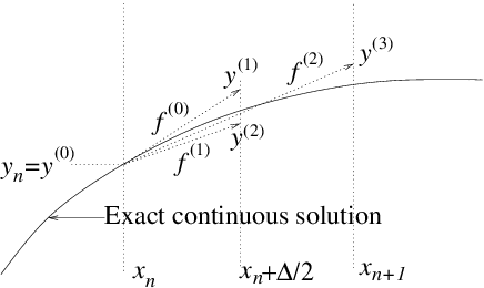
A Runge-Kutta method consists of taking a series of steps, each one of
which uses the estimate of the derivative function obtained from the
previous one, and then taking some weighted average of their
derivatives. 
<div class="p"><!----></div>
<a id="tth_fIg2.4">
</a>   <div style="text-align:center">  <img src="figures/rungekutta.png" alt="figures/rungekutta.png" /><a id="rungekutta">
</a>
  
<div style="text-align:center">Figure 2.4: Runge-Kutta fourth-order scheme with four partial steps,
    evaluates the derivative function <math xmlns="http://www.w3.org/1998/Math/MathML">
<mrow>
<msup><mrow><mi>f</mi></mrow><mrow><mo stretchy="false">(</mo><mi>k</mi><mo stretchy="false">)</mo></mrow>
</msup>
</mrow></math> with <math xmlns="http://www.w3.org/1998/Math/MathML">
<mrow><mi>k</mi><mo>=</mo><mn>0</mn><mo>,</mo><mn>1</mn><mo>,</mo><mn>2</mn><mo>,</mo><mn>3</mn></mrow></math>, at
    four places <math xmlns="http://www.w3.org/1998/Math/MathML">
<mrow><mo stretchy="false">(</mo>
<msub><mrow><mi>x</mi></mrow><mrow><mi>k</mi></mrow>
</msub>
<mo>,</mo>
<msub><mrow><mi>y</mi></mrow><mrow><mi>k</mi></mrow>
</msub>
<mo stretchy="false">)</mo></mrow></math>, each determined by extrapolation along
    the previous derivative.<a id="rungekutta">
</a></div>
</div>
<div class="p"><!----></div>
Specifically, the <em>fourth-order (accurate)
  Runge-Kutta</em><a 
id="fourth-order22117"></a> scheme, which is by far the most
popular and is illustrated in Fig.&nbsp;<a href="chap2.xml#rungekutta">2.4</a>, uses:
<a id="ode17a">
</a><br />
<table width="100%"><tr><td align="center">
    <math xmlns="http://www.w3.org/1998/Math/MathML">
    <mstyle displaystyle="true"><mrow>
<mtable displaystyle="true" align="right" width="80%">
<mtr><mtd columnalign="right" columnspan="1"><mrow>
<msup><mrow><mi>f</mi></mrow><mrow><mo stretchy="false">(</mo><mn>0</mn><mo stretchy="false">)</mo></mrow>
</msup>
</mrow>
</mtd><mtd columnalign="left">
<mrow><mo>=</mo></mrow>
</mtd><mtd columnalign="left">
<mrow><mi>f</mi><mo stretchy="false">(</mo>
<msub><mrow><mi>y</mi></mrow><mrow><mi>n</mi></mrow>
</msub>
<mo>,</mo>
<msub><mrow><mi>x</mi></mrow><mrow><mi>n</mi></mrow>
</msub>
<mo stretchy="false">)</mo></mrow>
</mtd></mtr>
<mtr><mtd columnalign="right" columnspan="1"><mrow>
<msup><mrow><mi>f</mi></mrow><mrow><mo stretchy="false">(</mo><mn>1</mn><mo stretchy="false">)</mo></mrow>
</msup>
</mrow>
</mtd><mtd columnalign="left">
<mrow><mo>=</mo></mrow>
</mtd><mtd columnalign="left">
<mrow><mi>f</mi><mo stretchy="false">(</mo>
<msub><mrow><mi>y</mi></mrow><mrow><mi>n</mi></mrow>
</msub>
<mo>+</mo>
<msup><mrow><mi>f</mi></mrow><mrow><mo stretchy="false">(</mo><mn>0</mn><mo stretchy="false">)</mo></mrow>
</msup>

<mfrac><mrow><mi mathvariant="italic">&Delta;</mi></mrow>
<mrow><mn>2</mn></mrow>
</mfrac>
<mo>,</mo>
<msub><mrow><mi>x</mi></mrow><mrow><mi>n</mi></mrow>
</msub>
<mo>+</mo>
<mfrac><mrow><mi mathvariant="italic">&Delta;</mi></mrow>
<mrow><mn>2</mn></mrow>
</mfrac>
<mo stretchy="false">)</mo></mrow>
</mtd></mtr>
<mtr><mtd columnalign="right" columnspan="1"><mrow>
<msup><mrow><mi>f</mi></mrow><mrow><mo stretchy="false">(</mo><mn>2</mn><mo stretchy="false">)</mo></mrow>
</msup>
</mrow>
</mtd><mtd columnalign="left">
<mrow><mo>=</mo></mrow>
</mtd><mtd columnalign="left">
<mrow><mi>f</mi><mo stretchy="false">(</mo>
<msub><mrow><mi>y</mi></mrow><mrow><mi>n</mi></mrow>
</msub>
<mo>+</mo>
<msup><mrow><mi>f</mi></mrow><mrow><mo stretchy="false">(</mo><mn>1</mn><mo stretchy="false">)</mo></mrow>
</msup>

<mfrac><mrow><mi mathvariant="italic">&Delta;</mi></mrow>
<mrow><mn>2</mn></mrow>
</mfrac>
<mo>,</mo>
<msub><mrow><mi>x</mi></mrow><mrow><mi>n</mi></mrow>
</msub>
<mo>+</mo>
<mfrac><mrow><mi mathvariant="italic">&Delta;</mi></mrow>
<mrow><mn>2</mn></mrow>
</mfrac>
<mo stretchy="false">)</mo></mrow>
</mtd><mtd columnalign="right">&emsp;&emsp;&emsp;&emsp;&emsp;&emsp;<mo stretchy="false">(</mo><mn>2</mn><mo>.</mo><mn>16</mn><mo stretchy="false">)</mo></mtd></mtr>
<mtr><mtd columnalign="right" columnspan="1"><mrow>
<msup><mrow><mi>f</mi></mrow><mrow><mo stretchy="false">(</mo><mn>3</mn><mo stretchy="false">)</mo></mrow>
</msup>
</mrow>
</mtd><mtd columnalign="left">
<mrow><mo>=</mo></mrow>
</mtd><mtd columnalign="left">
<mrow><mi>f</mi><mo stretchy="false">(</mo>
<msub><mrow><mi>y</mi></mrow><mrow><mi>n</mi></mrow>
</msub>
<mo>+</mo>
<msup><mrow><mi>f</mi></mrow><mrow><mo stretchy="false">(</mo><mn>2</mn><mo stretchy="false">)</mo></mrow>
</msup>
<mi mathvariant="italic">&Delta;</mi><mo>,</mo>
<msub><mrow><mi>x</mi></mrow><mrow><mi>n</mi></mrow>
</msub>
<mo>+</mo><mi mathvariant="italic">&Delta;</mi><mo stretchy="false">)</mo><mo>,</mo></mrow>
</mtd></mtr>
</mtable>
</mrow>
    </mstyle></math>
</td></tr></table>
<br />

in which two steps are to the half-way point <math xmlns="http://www.w3.org/1998/Math/MathML">
<mrow>
<mfrac><mrow><mi mathvariant="italic">&Delta;</mi></mrow>
<mrow><mn>2</mn></mrow>
</mfrac>
</mrow></math>.
Then the following combination
<a id="ode18">
</a><br />
<table width="100%"><tr><td align="center">
    <math xmlns="http://www.w3.org/1998/Math/MathML">
    <mstyle displaystyle="true"><mrow>
<msub><mrow><mi>y</mi></mrow><mrow><mi>n</mi><mo>+</mo><mn>1</mn></mrow>
</msub>
<mo>=</mo>
<msub><mrow><mi>y</mi></mrow><mrow><mi>n</mi></mrow>
</msub>
<mo>+</mo><mo stretchy="false">(</mo>
<mfrac><mrow>
<msup><mrow><mi>f</mi></mrow><mrow><mo stretchy="false">(</mo><mn>0</mn><mo stretchy="false">)</mo></mrow>
</msup>
</mrow>
<mrow><mn>6</mn></mrow>
</mfrac>
<mo>+</mo>
<mfrac><mrow>
<msup><mrow><mi>f</mi></mrow><mrow><mo stretchy="false">(</mo><mn>1</mn><mo stretchy="false">)</mo></mrow>
</msup>
</mrow>
<mrow><mn>3</mn></mrow>
</mfrac>
<mo>+</mo>
<mfrac><mrow>
<msup><mrow><mi>f</mi></mrow><mrow><mo stretchy="false">(</mo><mn>2</mn><mo stretchy="false">)</mo></mrow>
</msup>
</mrow>
<mrow><mn>3</mn></mrow>
</mfrac>
<mo>+</mo>
<mfrac><mrow>
<msup><mrow><mi>f</mi></mrow><mrow><mo stretchy="false">(</mo><mn>3</mn><mo stretchy="false">)</mo></mrow>
</msup>
</mrow>
<mrow><mn>6</mn></mrow>
</mfrac>
<mo stretchy="false">)</mo><mi mathvariant="italic">&Delta;</mi><mo>+</mo><mi>O</mi><mo stretchy="false">(</mo>
<msup><mrow><mi mathvariant="italic">&Delta;</mi></mrow><mrow><mn>5</mn></mrow>
</msup>
<mo stretchy="false">)</mo><mo>,</mo></mrow>
    </mstyle></math></td><td width="1">
    <math xmlns="http://www.w3.org/1998/Math/MathML">
    <mstyle displaystyle="true"><mrow><mo stretchy="false">(</mo><mn>2</mn><mo>.</mo><mn>17</mn><mo stretchy="false">)</mo></mrow>
    </mstyle></math>
</td></tr></table>


gives an approximation accurate to fourth-order<a href="footnote.xml#tthFtNtABF" id="tthFrefABF"><math xmlns="http://www.w3.org/1998/Math/MathML">
<mrow>
<msup><mrow></mrow><mrow><mn>15</mn></mrow>
</msup>
</mrow></math></a>

<div class="p"><!----></div>
The Runge-Kutta method costs more computation per step, because it
requires four evaluations of the function <math xmlns="http://www.w3.org/1998/Math/MathML">
<mrow><mi>f</mi><mo stretchy="false">(</mo><mi>y</mi><mo>,</mo><mi>x</mi><mo stretchy="false">)</mo></mrow></math>, rather than just
one. But that is often more than compensated by the ability to take
larger steps than with the Euler method for the same accuracy.

<div class="p"><!----></div>
     <a id="tth_sEc2.2.3"></a><h3>
2.2.3&nbsp;&nbsp;Stability</h3>

<div class="p"><!----></div>
<a 
id="stability_of_ODE_solution22118"></a><a 
id="stability22119"></a>The second, and possibly more important, weakness of explicit<a 
id="explicit22120"></a>
integration is in respect of stability. Consider a linear differential
equation 
<a id="ode19">
</a><br />
<table width="100%"><tr><td align="center">
    <math xmlns="http://www.w3.org/1998/Math/MathML">
    <mstyle displaystyle="true"><mrow>
<mfrac><mrow><mi mathvariant="italic">dy</mi></mrow>
<mrow><mi mathvariant="italic">dx</mi></mrow>
</mfrac>
<mo>=</mo><mo>-</mo><mi>k</mi><mi>y</mi><mo>,</mo></mrow>
    </mstyle></math></td><td width="1">
    <math xmlns="http://www.w3.org/1998/Math/MathML">
    <mstyle displaystyle="true"><mrow><mo stretchy="false">(</mo><mn>2</mn><mo>.</mo><mn>18</mn><mo stretchy="false">)</mo></mrow>
    </mstyle></math>
</td></tr></table>


where <math xmlns="http://www.w3.org/1998/Math/MathML">
<mrow><mi>k</mi></mrow></math> is a positive constant.
This of course has the solution <math xmlns="http://www.w3.org/1998/Math/MathML">
<mrow><mi>y</mi><mo>=</mo>
<msub><mrow><mi>y</mi></mrow><mrow><mn>0</mn></mrow>
</msub>
<mi>exp</mi><mo stretchy="false">(</mo><mo>-</mo><mi>k</mi><mi>x</mi><mo stretchy="false">)</mo></mrow></math>. But suppose
we integrate it numerically using the explicit scheme
<a id="ode20">
</a><br />
<table width="100%"><tr><td align="center">
    <math xmlns="http://www.w3.org/1998/Math/MathML">
    <mstyle displaystyle="true"><mrow>
<msub><mrow><mi>y</mi></mrow><mrow><mi>n</mi><mo>+</mo><mn>1</mn></mrow>
</msub>
<mo>=</mo>
<msub><mrow><mi>y</mi></mrow><mrow><mi>n</mi></mrow>
</msub>
<mo>+</mo><mi>f</mi><mo stretchy="false">(</mo>
<msub><mrow><mi>y</mi></mrow><mrow><mi>n</mi></mrow>
</msub>
<mo>,</mo>
<msub><mrow><mi>x</mi></mrow><mrow><mi>n</mi></mrow>
</msub>
<mo stretchy="false">)</mo><mo stretchy="false">(</mo>
<msub><mrow><mi>x</mi></mrow><mrow><mi>n</mi><mo>+</mo><mn>1</mn></mrow>
</msub>
<mo>-</mo>
<msub><mrow><mi>x</mi></mrow><mrow><mi>n</mi></mrow>
</msub>
<mo stretchy="false">)</mo><mo>=</mo>
<msub><mrow><mi>y</mi></mrow><mrow><mi>n</mi></mrow>
</msub>
<mo stretchy="false">(</mo><mn>1</mn><mo>-</mo><mi>k</mi><mi mathvariant="italic">&Delta;</mi><mo stretchy="false">)</mo><mo>.</mo></mrow>
    </mstyle></math></td><td width="1">
    <math xmlns="http://www.w3.org/1998/Math/MathML">
    <mstyle displaystyle="true"><mrow><mo stretchy="false">(</mo><mn>2</mn><mo>.</mo><mn>19</mn><mo stretchy="false">)</mo></mrow>
    </mstyle></math>
</td></tr></table>


This finite difference equation<a 
id="finite_difference22121"></a> has the solution
<a id="ode21">
</a><br />
<table width="100%"><tr><td align="center">
    <math xmlns="http://www.w3.org/1998/Math/MathML">
    <mstyle displaystyle="true"><mrow>
<msub><mrow><mi>y</mi></mrow><mrow><mi>n</mi></mrow>
</msub>
<mo>=</mo>
<msub><mrow><mi>y</mi></mrow><mrow><mn>0</mn></mrow>
</msub>
<mo stretchy="false">(</mo><mn>1</mn><mo>-</mo><mi>k</mi><mi mathvariant="italic">&Delta;</mi>
<msup><mrow><mo stretchy="false">)</mo></mrow><mrow><mi>n</mi></mrow>
</msup>
<mo>,</mo></mrow>
    </mstyle></math></td><td width="1">
    <math xmlns="http://www.w3.org/1998/Math/MathML">
    <mstyle displaystyle="true"><mrow><mo stretchy="false">(</mo><mn>2</mn><mo>.</mo><mn>20</mn><mo stretchy="false">)</mo></mrow>
    </mstyle></math>
</td></tr></table>


as may be verified by the simple observation that
<math xmlns="http://www.w3.org/1998/Math/MathML">
<mrow>
<msub><mrow><mi>y</mi></mrow><mrow><mi>n</mi><mo>+</mo><mn>1</mn></mrow>
</msub>
<mo stretchy="false">/</mo>
<msub><mrow><mi>y</mi></mrow><mrow><mi>n</mi></mrow>
</msub>
<mo>=</mo><mo stretchy="false">(</mo><mn>1</mn><mo>-</mo><mi>k</mi><mi mathvariant="italic">&Delta;</mi><mo stretchy="false">)</mo></mrow></math>. (This ratio is called the amplification
factor<a 
id="amplification_factor22122"></a>.) If <math xmlns="http://www.w3.org/1998/Math/MathML">
<mrow><mi>k</mi><mi mathvariant="italic">&Delta;</mi></mrow></math> is a small number,
then no difficulties will arise, and our scheme will produce
approximately correct results. However, a choice <math xmlns="http://www.w3.org/1998/Math/MathML">
<mrow><mi>k</mi><mi mathvariant="italic">&Delta;</mi><mo>&gt;</mo><mn>2</mn></mrow></math>
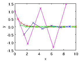
compromises not only accuracy, but also <em>stability</em>. The
resulting solution has alternating sign; it oscillates; but also its
magnitude <em>increases</em> with <math xmlns="http://www.w3.org/1998/Math/MathML">
<mrow><mi>n</mi></mrow></math> and will tend to infinity at large
<math xmlns="http://www.w3.org/1998/Math/MathML">
<mrow><mi>x</mi></mrow></math>. It has become unstable, as illustrated in Fig.&nbsp;<a href="chap2.xml#unstable1d">2.5</a>.

<div class="p"><!----></div>
<a id="tth_fIg2.5">
</a>   <img src="figures/unstable1d.png" alt="figures/unstable1d.png" /><a id="unstable1d">
</a>
  
<div style="text-align:center">Figure 2.5: Explicit numerical integration of eq.&nbsp;(<a href="chap2.xml#ode19">2.18</a>), using eq.&nbsp;    (<a href="chap2.xml#ode20">2.19</a>) leads to an oscillatory instability if the step
    length is too long. Four step lengths are shown <math xmlns="http://www.w3.org/1998/Math/MathML">
<mrow><mi>k</mi><mi mathvariant="italic">&Delta;</mi><mo>=</mo><mn>0</mn><mo>.</mo><mn>5</mn><mo>,</mo><mn>0</mn><mo>.</mo><mn>9</mn><mo>,</mo><mn>1</mn><mo>.</mo><mn>5</mn><mo>,</mo><mn>2</mn><mo>.</mo><mn>1</mn></mrow></math>.<a id="unstable1d">
</a></div>

<div class="p"><!----></div>
In general, an explicit discrete advancing scheme requires the step in
the independent variable to be less than some value (in this case
<math xmlns="http://www.w3.org/1998/Math/MathML">
<mrow><mn>2</mn><mo stretchy="false">/</mo><mi>k</mi></mrow></math>) in order to achieve stability. 

<div class="p"><!----></div>
An <em>implicit</em><a 
id="implicit22123"></a> advancing scheme, by contrast, is one in which the
value of the derivative used to advance the variable is taken at the
<em>end</em> of the step rather than at the <em>beginning</em>. For our
example equation, this would be a numerical scheme of the form
<a id="ode22">
</a><br />
<table width="100%"><tr><td align="center">
    <math xmlns="http://www.w3.org/1998/Math/MathML">
    <mstyle displaystyle="true"><mrow>
<msub><mrow><mi>y</mi></mrow><mrow><mi>n</mi><mo>+</mo><mn>1</mn></mrow>
</msub>
<mo>=</mo>
<msub><mrow><mi>y</mi></mrow><mrow><mi>n</mi></mrow>
</msub>
<mo>+</mo><mi>f</mi><mo stretchy="false">(</mo>
<msub><mrow><mi>y</mi></mrow><mrow><mi>n</mi><mo>+</mo><mn>1</mn></mrow>
</msub>
<mo>,</mo>
<msub><mrow><mi>x</mi></mrow><mrow><mi>n</mi><mo>+</mo><mn>1</mn></mrow>
</msub>
<mo stretchy="false">)</mo><mo stretchy="false">(</mo>
<msub><mrow><mi>x</mi></mrow><mrow><mi>n</mi><mo>+</mo><mn>1</mn></mrow>
</msub>
<mo>-</mo>
<msub><mrow><mi>x</mi></mrow><mrow><mi>n</mi></mrow>
</msub>
<mo stretchy="false">)</mo><mo>=</mo>
<msub><mrow><mi>y</mi></mrow><mrow><mi>n</mi></mrow>
</msub>
<mo>-</mo><mi>k</mi>
<msub><mrow><mi>y</mi></mrow><mrow><mi>n</mi><mo>+</mo><mn>1</mn></mrow>
</msub>
<mi mathvariant="italic">&Delta;</mi><mo>.</mo></mrow>
    </mstyle></math></td><td width="1">
    <math xmlns="http://www.w3.org/1998/Math/MathML">
    <mstyle displaystyle="true"><mrow><mo stretchy="false">(</mo><mn>2</mn><mo>.</mo><mn>21</mn><mo stretchy="false">)</mo></mrow>
    </mstyle></math>
</td></tr></table>


It is easy to rearrange this equation into
<a id="ode23">
</a><br />
<table width="100%"><tr><td align="center">
    <math xmlns="http://www.w3.org/1998/Math/MathML">
    <mstyle displaystyle="true"><mrow>
<msub><mrow><mi>y</mi></mrow><mrow><mi>n</mi><mo>+</mo><mn>1</mn></mrow>
</msub>
<mo stretchy="false">(</mo><mn>1</mn><mo>+</mo><mi>k</mi><mi mathvariant="italic">&Delta;</mi><mo stretchy="false">)</mo><mo>=</mo>
<msub><mrow><mi>y</mi></mrow><mrow><mi>n</mi></mrow>
</msub>
<mo>.</mo></mrow>
    </mstyle></math></td><td width="1">
    <math xmlns="http://www.w3.org/1998/Math/MathML">
    <mstyle displaystyle="true"><mrow><mo stretchy="false">(</mo><mn>2</mn><mo>.</mo><mn>22</mn><mo stretchy="false">)</mo></mrow>
    </mstyle></math>
</td></tr></table>


This has solution
<a id="ode24">
</a><br />
<table width="100%"><tr><td align="center">
    <math xmlns="http://www.w3.org/1998/Math/MathML">
    <mstyle displaystyle="true"><mrow>
<msub><mrow><mi>y</mi></mrow><mrow><mi>n</mi></mrow>
</msub>
<mo>=</mo>
<msub><mrow><mi>y</mi></mrow><mrow><mn>0</mn></mrow>
</msub>
<mo stretchy="false">(</mo><mn>1</mn><mo>+</mo><mi>k</mi><mi mathvariant="italic">&Delta;</mi>
<msup><mrow><mo stretchy="false">)</mo></mrow><mrow><mo>-</mo><mi>n</mi></mrow>
</msup>
<mo>.</mo></mrow>
    </mstyle></math></td><td width="1">
    <math xmlns="http://www.w3.org/1998/Math/MathML">
    <mstyle displaystyle="true"><mrow><mo stretchy="false">(</mo><mn>2</mn><mo>.</mo><mn>23</mn><mo stretchy="false">)</mo></mrow>
    </mstyle></math>
</td></tr></table>


For positive <math xmlns="http://www.w3.org/1998/Math/MathML">
<mrow><mi>k</mi><mi mathvariant="italic">&Delta;</mi></mrow></math> (the case of interest) this finite difference
equation <em>never</em> becomes unstable, no matter how big <math xmlns="http://www.w3.org/1998/Math/MathML">
<mrow><mi>k</mi><mi mathvariant="italic">&Delta;</mi></mrow></math>
is, because the solution consists of successive powers of an
amplification factor <math xmlns="http://www.w3.org/1998/Math/MathML">
<mrow><mn>1</mn><mo stretchy="false">/</mo><mo stretchy="false">(</mo><mn>1</mn><mo>+</mo><mi>k</mi><mi mathvariant="italic">&Delta;</mi><mo stretchy="false">)</mo></mrow></math> whose magnitude is always less
than 1. This is a characteristic of implicit
schemes<a 
id="implicit_schemes22124"></a>. They are generally stable even for
large steps<a 
id="step_size22125"></a>.

<div class="p"><!----></div>
 <a id="tth_sEc2.3"></a><h2>
2.3&nbsp;&nbsp;Multidimensional Stiff Equations: Implicit Schemes</h2>
<a id="StiffStability">
</a>

<div class="p"><!----></div>
<a 
id="stiff_equations23126"></a>The question of stability for an order-one system (the scalar problem)
is generally not very interesting; because instability of the explicit
scheme occurs only when the step size is longer than the
characteristic spatial scale of the problem <math xmlns="http://www.w3.org/1998/Math/MathML">
<mrow><mn>1</mn><mo stretchy="false">/</mo><mi>k</mi></mrow></math>. If you've
chosen your step size so large, you are already failing to get an
accurate solution of the equation. However, multidimensional (i.e.&nbsp;higher order) sets of (vector) equations may have multiple solutions
that have very different scale-lengths in the independent variable.  A
classic example is an order-two homogeneous linear system with constant
coefficients
<a id="ode25">
</a><br />
<table width="100%"><tr><td align="center">
    <math xmlns="http://www.w3.org/1998/Math/MathML">
    <mstyle displaystyle="true"><mrow>
<mfrac><mrow><mi>d</mi></mrow>
<mrow><mi mathvariant="italic">dx</mi></mrow>
</mfrac>
<mi mathvariant="bold">y</mi><mo>=</mo><mi mathvariant="bold">A</mi><mi mathvariant="bold">y</mi><mo>,</mo><mi>&emsp;&emsp;&emsp;</mi>
<mtext>where for example</mtext>
<mi>&emsp;&emsp;&emsp;</mi><mi mathvariant="bold">A</mi><mo>=</mo><mrow><mo>(</mo>
<mtable>
<mtr><mtd columnalign="center"><mrow><mn>0</mn></mrow></mtd><mtd columnalign="center"><mrow><mo>-</mo><mn>1</mn></mrow></mtd></mtr>
<mtr><mtd columnalign="center"><mrow><mn>100</mn></mrow></mtd><mtd columnalign="center"><mrow><mo>-</mo><mn>101</mn></mrow></mtd></mtr></mtable>

<mo>)</mo></mrow><mo>.</mo></mrow>
    </mstyle></math></td><td width="1">
    <math xmlns="http://www.w3.org/1998/Math/MathML">
    <mstyle displaystyle="true"><mrow><mo stretchy="false">(</mo><mn>2</mn><mo>.</mo><mn>24</mn><mo stretchy="false">)</mo></mrow>
    </mstyle></math>
</td></tr></table>


For any such linear system the solution can be constructed by
consideration of the <em>eigenvalues</em><a 
id="eigenvalue23127"></a> of the
matrix <math xmlns="http://www.w3.org/1998/Math/MathML">
<mrow><mi mathvariant="bold">A</mi></mrow></math>: those numbers for which there exists a solution to
<math xmlns="http://www.w3.org/1998/Math/MathML">
<mrow><mi mathvariant="bold">A</mi><mi mathvariant="bold">y</mi><mo>=</mo><mi mathvariant="italic">&lambda;</mi><mi mathvariant="bold">y</mi></mrow></math>.  If these are <math xmlns="http://www.w3.org/1998/Math/MathML">
<mrow>
<msub><mrow><mi mathvariant="italic">&lambda;</mi></mrow><mrow><mi>j</mi></mrow>
</msub>
</mrow></math> and the
corresponding eigenvectors<a 
id="eigenvector23128"></a> are <math xmlns="http://www.w3.org/1998/Math/MathML">
<mrow>
<msub><mrow><mi mathvariant="bold">y</mi></mrow><mrow><mi>j</mi></mrow>
</msub>
</mrow></math>, then
<math xmlns="http://www.w3.org/1998/Math/MathML">
<mrow><mi mathvariant="bold">y</mi><mo>=</mo>
<msub><mrow><mi mathvariant="bold">y</mi></mrow><mrow><mi>j</mi></mrow>
</msub>
<mi>exp</mi><mo stretchy="false">(</mo>
<msub><mrow><mi mathvariant="italic">&lambda;</mi></mrow><mrow><mi>j</mi></mrow>
</msub>
<mi>x</mi><mo stretchy="false">)</mo></mrow></math> are solutions to the
equation. The complete solution can be constructed as a sum of these
different characteristic solutions, weighted by coefficients to
satisfy the initial conditions.  The point of our particular example
matrix is that its eignvalues are -100 and -1. Consequently in order
to integrate numerically a solution that has a significant quantity of
the second, slowly changing, solution <math xmlns="http://www.w3.org/1998/Math/MathML">
<mrow>
<msub><mrow><mi mathvariant="italic">&lambda;</mi></mrow><mrow><mn>2</mn></mrow>
</msub>
<mo>=</mo><mo>-</mo><mn>1</mn></mrow></math>, it is necessary
nevertheless to ensure the stability of the first, rapidly changing,
solution, <math xmlns="http://www.w3.org/1998/Math/MathML">
<mrow>
<msub><mrow><mi mathvariant="italic">&lambda;</mi></mrow><mrow><mn>1</mn></mrow>
</msub>
<mo>=</mo><mo>-</mo><mn>100</mn></mrow></math>. Otherwise, if the first solutions is
unstable, no matter how little of that solution we start with, it will
eventually grow exponentially large and erroneously dominate our
result. If an explicit advancing scheme is used, then stability
requires <math xmlns="http://www.w3.org/1998/Math/MathML">
<mrow><mo stretchy="false">&verbar;</mo>
<msub><mrow><mi mathvariant="italic">&lambda;</mi></mrow><mrow><mn>1</mn></mrow>
</msub>
<mo stretchy="false">&verbar;</mo><mi mathvariant="italic">&Delta;</mi><mo>&lt;</mo><mn>2</mn></mrow></math> as well as <math xmlns="http://www.w3.org/1998/Math/MathML">
<mrow><mo stretchy="false">&verbar;</mo>
<msub><mrow><mi mathvariant="italic">&lambda;</mi></mrow><mrow><mn>2</mn></mrow>
</msub>
<mo stretchy="false">&verbar;</mo><mi mathvariant="italic">&Delta;</mi><mo>&lt;</mo><mn>2</mn></mrow></math>, and
the <math xmlns="http://www.w3.org/1998/Math/MathML">
<mrow>
<msub><mrow><mi mathvariant="italic">&lambda;</mi></mrow><mrow><mn>1</mn></mrow>
</msub>
</mrow></math> condition is by far the most restrictive.  There are then at
least <math xmlns="http://www.w3.org/1998/Math/MathML">
<mrow><mo>~</mo><mo stretchy="false">&verbar;</mo>
<msub><mrow><mi mathvariant="italic">&lambda;</mi></mrow><mrow><mn>1</mn></mrow>
</msub>
<mo stretchy="false">/</mo>
<msub><mrow><mi mathvariant="italic">&lambda;</mi></mrow><mrow><mn>2</mn></mrow>
</msub>
<mo stretchy="false">&verbar;</mo></mrow></math> steps during the decay of the
(<math xmlns="http://www.w3.org/1998/Math/MathML">
<mrow>
<msub><mrow><mi mathvariant="italic">&lambda;</mi></mrow><mrow><mn>2</mn></mrow>
</msub>
</mrow></math>) solution of interest. Because this ratio is large, an
explicit scheme is computationally expensive, requiring many steps. In
general, the <em>stiffness</em><a 
id="stiffness23129"></a> of a differential
equation system can be measured by the ratio of the largest to the
smallest eigenvalue magnitude. If this ratio is large, the system is
stiff, and that means it is hard to integrate explicitly.

<div class="p"><!----></div>
Using an implicit scheme avoids the necessity for taking very small
steps. It does so at the cost of solving the matrix problem <math xmlns="http://www.w3.org/1998/Math/MathML">
<mrow><mo stretchy="false">(</mo><mi mathvariant="bold">I</mi><mo>-</mo><mi mathvariant="italic">&Delta;</mi><mo>.</mo><mi mathvariant="bold">A</mi><mo stretchy="false">)</mo>
<msub><mrow><mi mathvariant="bold">y</mi></mrow><mrow><mi>n</mi><mo>+</mo><mn>1</mn></mrow>
</msub>
<mo>=</mo>
<msub><mrow><mi mathvariant="bold">y</mi></mrow><mrow><mi>n</mi></mrow>
</msub>
</mrow></math>.  This requires the
inversion<a 
id="matrix_inversion23130"></a> of a matrix in order to evaluate
<a id="ode26">
</a><br />
<table width="100%"><tr><td align="center">
    <math xmlns="http://www.w3.org/1998/Math/MathML">
    <mstyle displaystyle="true"><mrow>
<msub><mrow><mi mathvariant="bold">y</mi></mrow><mrow><mi>n</mi><mo>+</mo><mn>1</mn></mrow>
</msub>
<mo>=</mo><mo stretchy="false">(</mo><mi mathvariant="bold">I</mi><mo>-</mo><mi mathvariant="italic">&Delta;</mi><mo>.</mo><mi mathvariant="bold">A</mi>
<msup><mrow><mo stretchy="false">)</mo></mrow><mrow><mo>-</mo><mn>1</mn></mrow>
</msup>

<msub><mrow><mi mathvariant="bold">y</mi></mrow><mrow><mi>n</mi></mrow>
</msub>
<mo>.</mo></mrow>
    </mstyle></math></td><td width="1">
    <math xmlns="http://www.w3.org/1998/Math/MathML">
    <mstyle displaystyle="true"><mrow><mo stretchy="false">(</mo><mn>2</mn><mo>.</mo><mn>25</mn><mo stretchy="false">)</mo></mrow>
    </mstyle></math>
</td></tr></table>


For a linear problem like the one we are considering, the single
inversion, done once and for all, is a relatively small cost compared
with the gain obtained by being able to take decent length steps. 

<div class="p"><!----></div>
All of this probably seems rather elaborate for a linear, constant
coefficient, system, since we are actually able to solve it
analytically when we know the eigenvalues and eigenvectors. However,
it becomes much more significant when we realize that the stability of
a <em>nonlinear</em><a 
id="nonlinear_stability23131"></a> system, or one in which
the coefficients vary with <math xmlns="http://www.w3.org/1998/Math/MathML">
<mrow><mi>x</mi></mrow></math> or <math xmlns="http://www.w3.org/1998/Math/MathML">
<mrow><mi>y</mi></mrow></math>, for which numerical integration
may be essential, is generally very well described by expressing it
approximately as a linear system<a 
id="linearization23132"></a> in the
neighborhood of the region under consideration, and then evaluating
the stability of the linearized system. The matrix that arises from
linearization when the (vectorial) derivative function is
<math xmlns="http://www.w3.org/1998/Math/MathML">
<mrow><mi mathvariant="bold">f</mi><mo stretchy="false">(</mo><mi mathvariant="bold">y</mi><mo>,</mo><mi>x</mi><mo stretchy="false">)</mo></mrow></math> has the elements <math xmlns="http://www.w3.org/1998/Math/MathML">
<mrow>
<msub><mrow><mi>A</mi></mrow><mrow><mi mathvariant="italic">ij</mi></mrow>
</msub>
<mo>=</mo><mo>&part;</mo>
<msub><mrow><mi>f</mi></mrow><mrow><mi>i</mi></mrow>
</msub>
<mo stretchy="false">/</mo><mo>&part;</mo>
<msub><mrow><mi>y</mi></mrow><mrow><mi>j</mi></mrow>
</msub>
</mrow></math>.  An implicit solution then requires <math xmlns="http://www.w3.org/1998/Math/MathML">
<mrow><mo stretchy="false">(</mo><mi mathvariant="bold">I</mi><mo>-</mo><mi mathvariant="italic">&Delta;</mi><mo>.</mo><mi mathvariant="bold">A</mi><mo stretchy="false">)</mo></mrow></math> to
be inverted for every step, because it is changing with position (if
the derivative function is nonlinear).

<div class="p"><!----></div>
In short, implicit schemes lead to greater stability, which is very
important with stiff systems, but require matrix inversion.

<div class="p"><!----></div>
 <a id="tth_sEc2.4"></a><h2>
2.4&nbsp;&nbsp;Leap-Frog Schemes</h2>

<div class="p"><!----></div>
<a 
id="Leap-Frog_scheme24133"></a> Codes such as
particle-in-cell<a 
id="PIC24134"></a><a 
id="particle-in-cell24135"></a> simulations of
plasmas, atomistic simulation<a 
id="atomistic_simulation24136"></a>, or any
codes that do large amount of orbit
integration<a 
id="orbit_integration24137"></a>, generally want to use as cheap a
scheme as possible to maintain their speed. The step size is often
dictated by questions other than the accuracy of the orbit
integration. In such situations, Runge-Kutta or implicit schemes are
rarely used. Instead, an accurate orbit integration can be obtained by
recognizing that Newton's second law of motion (acceleration
proportional to force) is a second-order vector equation that can most
conveniently be split into two first-order vector equations involving
position, velocity, and acceleration. The velocity we want for the
equation governing the evolution of position, <math xmlns="http://www.w3.org/1998/Math/MathML">
<mrow><mi>d</mi><mi mathvariant="bold-italic">x</mi><mo stretchy="false">/</mo><mi mathvariant="italic">dt</mi><mo>=</mo><mi mathvariant="bold-italic">v</mi></mrow></math>,
is the average velocity during the motion between two positions. An
unbiassed estimate of that velocity is to take it to be the velocity
at the <em>center</em> of the position step. So if the times at which we
evaluate the position <math xmlns="http://www.w3.org/1998/Math/MathML">
<mrow>
<msub><mrow><mi mathvariant="bold-italic">x</mi></mrow><mrow><mi>n</mi></mrow>
</msub>
</mrow></math> of the particle are denoted <math xmlns="http://www.w3.org/1998/Math/MathML">
<mrow>
<msub><mrow><mi>t</mi></mrow><mrow><mi>n</mi></mrow>
</msub>
</mrow></math>,
then we want the velocity at time <math xmlns="http://www.w3.org/1998/Math/MathML">
<mrow><mo stretchy="false">(</mo>
<msub><mrow><mi>t</mi></mrow><mrow><mi>n</mi><mo>+</mo><mn>1</mn></mrow>
</msub>
<mo>+</mo>
<msub><mrow><mi>t</mi></mrow><mrow><mi>n</mi></mrow>
</msub>
<mo stretchy="false">)</mo><mo stretchy="false">/</mo><mn>2</mn></mrow></math>. We might call
this time <math xmlns="http://www.w3.org/1998/Math/MathML">
<mrow>
<msub><mrow><mi>t</mi></mrow><mrow><mi>n</mi><mo>+</mo><mn>1</mn><mo stretchy="false">/</mo><mn>2</mn></mrow>
</msub>
</mrow></math><a 
id="half-step_position__t__n_1_2__24138"></a> and the velocity
<math xmlns="http://www.w3.org/1998/Math/MathML">
<mrow>
<msub><mrow><mi mathvariant="bold-italic">v</mi></mrow><mrow><mi>n</mi><mo>+</mo><mn>1</mn><mo stretchy="false">/</mo><mn>2</mn></mrow>
</msub>
</mrow></math>. Also, the acceleration we want for the equation for
the evolution of velocity, <math xmlns="http://www.w3.org/1998/Math/MathML">
<mrow><mi>d</mi><mi mathvariant="bold-italic">v</mi><mo stretchy="false">/</mo><mi mathvariant="italic">dt</mi><mo>=</mo><mi mathvariant="bold-italic">a</mi></mrow></math>, is the average
acceleration between two velocities. If the velocities are represented
at <math xmlns="http://www.w3.org/1998/Math/MathML">
<mrow>
<msub><mrow><mi>t</mi></mrow><mrow><mi>n</mi><mo>-</mo><mn>1</mn><mo stretchy="false">/</mo><mn>2</mn></mrow>
</msub>
</mrow></math> and <math xmlns="http://www.w3.org/1998/Math/MathML">
<mrow>
<msub><mrow><mi>t</mi></mrow><mrow><mi>n</mi><mo>+</mo><mn>1</mn><mo stretchy="false">/</mo><mn>2</mn></mrow>
</msub>
</mrow></math>, then the time at which we want the
acceleration is <math xmlns="http://www.w3.org/1998/Math/MathML">
<mrow>
<msub><mrow><mi>t</mi></mrow><mrow><mi>n</mi></mrow>
</msub>
</mrow></math>, and we might call that acceleration
<math xmlns="http://www.w3.org/1998/Math/MathML">
<mrow>
<msub><mrow><mi mathvariant="bold-italic">a</mi></mrow><mrow><mi>n</mi></mrow>
</msub>
</mrow></math>.

<div class="p"><!----></div>
We can therefore construct an appropriate centered<a 
id="centered24139"></a>
integration scheme as follows starting from position <math xmlns="http://www.w3.org/1998/Math/MathML">
<mrow><mi>n</mi></mrow></math>. 
<div class="p"><!----></div>
<br />
<table>
<tr><td align="left">(1) </td><td width="0">Move the particles using
their velocities <math xmlns="http://www.w3.org/1998/Math/MathML">
<mrow>
<msub><mrow><mi mathvariant="bold-italic">v</mi></mrow><mrow><mi>n</mi><mo>+</mo><mn>1</mn><mo stretchy="false">/</mo><mn>2</mn></mrow>
</msub>
</mrow></math> to find the new positions
<math xmlns="http://www.w3.org/1998/Math/MathML">
<mrow>
<msub><mrow><mi mathvariant="bold-italic">x</mi></mrow><mrow><mi>n</mi><mo>+</mo><mn>1</mn></mrow>
</msub>
<mo>=</mo>
<msub><mrow><mi mathvariant="bold-italic">x</mi></mrow><mrow><mi>n</mi></mrow>
</msub>
<mo>+</mo>
<msub><mrow><mi mathvariant="bold-italic">v</mi></mrow><mrow><mi>n</mi><mo>+</mo><mn>1</mn><mo stretchy="false">/</mo><mn>2</mn></mrow>
</msub>
<mo stretchy="false">(</mo>
<msub><mrow><mi>t</mi></mrow><mrow><mi>n</mi><mo>+</mo><mn>1</mn></mrow>
</msub>
<mo>-</mo>
<msub><mrow><mi>t</mi></mrow><mrow><mi>n</mi></mrow>
</msub>
<mo stretchy="false">)</mo></mrow></math>; this is called
the drift step<a 
id="drift_step24140"></a>.</td></tr>
<tr><td align="left">(2) </td><td width="0">Accelerate the velocities using the accelerations
<math xmlns="http://www.w3.org/1998/Math/MathML">
<mrow>
<msub><mrow><mi mathvariant="bold-italic">a</mi></mrow><mrow><mi>n</mi><mo>+</mo><mn>1</mn></mrow>
</msub>
</mrow></math> evaluated at the new positions <math xmlns="http://www.w3.org/1998/Math/MathML">
<mrow>
<msub><mrow><mi mathvariant="bold-italic">x</mi></mrow><mrow><mi>n</mi><mo>+</mo><mn>1</mn></mrow>
</msub>
</mrow></math> to
obtain the new velocities
<math xmlns="http://www.w3.org/1998/Math/MathML">
<mrow>
<msub><mrow><mi mathvariant="bold-italic">v</mi></mrow><mrow><mi>n</mi><mo>+</mo><mn>3</mn><mo stretchy="false">/</mo><mn>2</mn></mrow>
</msub>
<mo>=</mo>
<msub><mrow><mi mathvariant="bold-italic">v</mi></mrow><mrow><mi>n</mi><mo>+</mo><mn>1</mn><mo stretchy="false">/</mo><mn>2</mn></mrow>
</msub>
<mo>+</mo>
<msub><mrow><mi mathvariant="bold-italic">a</mi></mrow><mrow><mi>n</mi><mo>+</mo><mn>1</mn></mrow>
</msub>
<mo stretchy="false">(</mo>
<msub><mrow><mi>t</mi></mrow><mrow><mi>n</mi><mo>+</mo><mn>3</mn><mo stretchy="false">/</mo><mn>2</mn></mrow>
</msub>
<mo>-</mo>
<msub><mrow><mi>t</mi></mrow><mrow><mi>n</mi><mo>+</mo><mn>1</mn><mo stretchy="false">/</mo><mn>2</mn></mrow>
</msub>
<mo stretchy="false">)</mo></mrow></math>;
this is called the kick step<a 
id="kick_step24141"></a>.</td></tr>
<tr><td align="left">(3) </td><td width="0">Repeat (1) and (2) for the next time
step <math xmlns="http://www.w3.org/1998/Math/MathML">
<mrow><mi>n</mi><mo>+</mo><mn>1</mn></mrow></math>, and so on. 
</td></tr></table>
<a 
id="staggered_values24142"></a>

<div class="p"><!----></div>
<br />Each of the drift and kick steps can be simple
explicit advances. But because the velocities are suitably
time-shifted relative to the positions and accelerations, the result
is <em>second-order accurate</em>. Such a scheme is called a Leap-Frog
scheme, in reference to the children's game where each of two players
alternately jumps over the back of the other in moving to the new
position. Velocity and position are jumping over one another in time;
they never land at the same time (or place). See Fig.&nbsp;<a href="chap2.xml#leapfrogl">2.6</a>.

<div class="p"><!----></div>
<a id="tth_fIg2.6">
</a>   <img src="figures/leapfrog.png" alt="figures/leapfrog.png" /><a id="leapfrog">
</a>
  
<div style="text-align:center">Figure 2.6: Staggered values for <math xmlns="http://www.w3.org/1998/Math/MathML">
<mrow><mi>x</mi></mrow></math> and <math xmlns="http://www.w3.org/1998/Math/MathML">
<mrow><mi>v</mi></mrow></math> are updated leap-frog
    style.<a id="leapfrogl">
</a></div>

<div class="p"><!----></div>
One trap for the unwary in a Leap-Frog scheme is the specification of
initial values<a 
id="initial_values_leap-frog24143"></a>. If we want to
calculate an orbit which has specified initial position <math xmlns="http://www.w3.org/1998/Math/MathML">
<mrow>
<msub><mrow><mi mathvariant="bold-italic">x</mi></mrow><mrow><mn>0</mn></mrow>
</msub>
</mrow></math>
and velocity <math xmlns="http://www.w3.org/1998/Math/MathML">
<mrow>
<msub><mrow><mi mathvariant="bold-italic">v</mi></mrow><mrow><mn>0</mn></mrow>
</msub>
</mrow></math> at time <math xmlns="http://www.w3.org/1998/Math/MathML">
<mrow><mi>t</mi><mo>=</mo>
<msub><mrow><mi>t</mi></mrow><mrow><mn>0</mn></mrow>
</msub>
</mrow></math>, then it is not sufficient
simply to put the velocity initially equal to the specified
<math xmlns="http://www.w3.org/1998/Math/MathML">
<mrow>
<msub><mrow><mi mathvariant="bold-italic">v</mi></mrow><mrow><mn>0</mn></mrow>
</msub>
</mrow></math>. That is because the first velocity, which governs the
position step from <math xmlns="http://www.w3.org/1998/Math/MathML">
<mrow>
<msub><mrow><mi>t</mi></mrow><mrow><mn>0</mn></mrow>
</msub>
</mrow></math> to <math xmlns="http://www.w3.org/1998/Math/MathML">
<mrow>
<msub><mrow><mi>t</mi></mrow><mrow><mn>1</mn></mrow>
</msub>
</mrow></math> is <em>not</em> <math xmlns="http://www.w3.org/1998/Math/MathML">
<mrow>
<msub><mrow><mi mathvariant="bold-italic">v</mi></mrow><mrow><mn>0</mn></mrow>
</msub>
</mrow></math>, but
<math xmlns="http://www.w3.org/1998/Math/MathML">
<mrow>
<msub><mrow><mi mathvariant="bold-italic">v</mi></mrow><mrow><mn>1</mn><mo stretchy="false">/</mo><mn>2</mn></mrow>
</msub>
</mrow></math>. To start the integration off correctly, therefore, we
must take a <em>half-step</em> in velocity by putting <math xmlns="http://www.w3.org/1998/Math/MathML">
<mrow>
<msub><mrow><mi mathvariant="bold-italic">v</mi></mrow><mrow><mn>1</mn><mo stretchy="false">/</mo><mn>2</mn></mrow>
</msub>
<mo>=</mo>
<msub><mrow><mi mathvariant="bold-italic">v</mi></mrow><mrow><mn>0</mn></mrow>
</msub>
<mo>+</mo>
<msub><mrow><mi mathvariant="bold-italic">a</mi></mrow><mrow><mn>0</mn></mrow>
</msub>
<mo stretchy="false">(</mo>
<msub><mrow><mi>t</mi></mrow><mrow><mn>1</mn></mrow>
</msub>
<mo>-</mo>
<msub><mrow><mi>t</mi></mrow><mrow><mn>0</mn></mrow>
</msub>
<mo stretchy="false">)</mo><mo stretchy="false">/</mo><mn>2</mn></mrow></math>, before beginning the standard
integration.

<div class="p"><!----></div>
Leap-Frog schemes generally possess important conservation properties
such as conservation of momentum<a 
id="conservation_properties24144"></a>, that
can be essential for realistic simulation with a large number of
particles.

<div class="p"><!----></div>

<h2>Worked Example: Stability of finite differences</h2>

<div class="p"><!----></div>
<a 
id="explicit24145"></a><a 
id="implicit24146"></a>Find the stability limits when solving by discrete finite differences of length
<math xmlns="http://www.w3.org/1998/Math/MathML">
<mrow><mi mathvariant="italic">&Delta;</mi></mrow></math>, using explicit or implicit schemes, the initial value equation
<a id="worksecond">
</a><br />
<table width="100%"><tr><td align="center">
    <math xmlns="http://www.w3.org/1998/Math/MathML">
    <mstyle displaystyle="true"><mrow>
<mfrac><mrow>
<msup><mrow><mi>d</mi></mrow><mrow><mn>2</mn></mrow>
</msup>
<mi>y</mi></mrow>
<mrow>
<msup><mrow><mi mathvariant="italic">dx</mi></mrow><mrow><mn>2</mn></mrow>
</msup>
</mrow>
</mfrac>
<mo>+</mo><mn>2</mn><mi mathvariant="italic">&alpha;</mi>
<mfrac><mrow><mi mathvariant="italic">dy</mi></mrow>
<mrow><mi mathvariant="italic">dx</mi></mrow>
</mfrac>
<mo>+</mo>
<msup><mrow><mi>k</mi></mrow><mrow><mn>2</mn></mrow>
</msup>
<mi>y</mi><mo>=</mo><mi>g</mi><mo stretchy="false">(</mo><mi>x</mi><mo stretchy="false">)</mo><mo>,</mo></mrow>
    </mstyle></math></td><td width="1">
    <math xmlns="http://www.w3.org/1998/Math/MathML">
    <mstyle displaystyle="true"><mrow><mo stretchy="false">(</mo><mn>2</mn><mo>.</mo><mn>26</mn><mo stretchy="false">)</mo></mrow>
    </mstyle></math>
</td></tr></table>


where <math xmlns="http://www.w3.org/1998/Math/MathML">
<mrow><mi mathvariant="italic">&alpha;</mi></mrow></math> is a positive constant <math xmlns="http://www.w3.org/1998/Math/MathML">
<mrow><mo>&lt;</mo><mo stretchy="false">&verbar;</mo><mi>k</mi><mo stretchy="false">&verbar;</mo></mrow></math>.
<div class="p"><!----></div>
<br />First, reduce the equation to standard first-order form by
writing<a 
id="order_reduction24147"></a>
<a id="wk2standard">
</a><br />
<table width="100%"><tr><td align="center">
    <math xmlns="http://www.w3.org/1998/Math/MathML">
    <mstyle displaystyle="true"><mrow>
<mfrac><mrow><mi>d</mi></mrow>
<mrow><mi mathvariant="italic">dx</mi></mrow>
</mfrac>
<mrow><mo>(</mo>
<mtable>
<mtr><mtd columnalign="center"><mrow>
<msup><mrow><mi>y</mi></mrow><mrow><mo stretchy="false">(</mo><mn>0</mn><mo stretchy="false">)</mo></mrow>
</msup>
</mrow></mtd></mtr>
<mtr><mtd columnalign="center"><mrow>
<msup><mrow><mi>y</mi></mrow><mrow><mo stretchy="false">(</mo><mn>1</mn><mo stretchy="false">)</mo></mrow>
</msup>
</mrow></mtd></mtr></mtable>

<mo>)</mo></mrow><mo>=</mo><mrow><mo>(</mo>
<mtable>
<mtr><mtd columnalign="center"><mrow>
<msup><mrow><mi>y</mi></mrow><mrow><mo stretchy="false">(</mo><mn>1</mn><mo stretchy="false">)</mo></mrow>
</msup>
</mrow></mtd></mtr>
<mtr><mtd columnalign="center"><mrow><mi>g</mi><mo stretchy="false">(</mo><mi>x</mi><mo stretchy="false">)</mo><mo>-</mo><mn>2</mn><mi mathvariant="italic">&alpha;</mi>
<msup><mrow><mi>y</mi></mrow><mrow><mo stretchy="false">(</mo><mn>1</mn><mo stretchy="false">)</mo></mrow>
</msup>
<mo>-</mo>
<msup><mrow><mi>k</mi></mrow><mrow><mn>2</mn></mrow>
</msup>

<msup><mrow><mi>y</mi></mrow><mrow><mo stretchy="false">(</mo><mn>0</mn><mo stretchy="false">)</mo></mrow>
</msup>
</mrow></mtd></mtr></mtable>

<mo>)</mo></mrow><mo>=</mo><mrow><mo>(</mo>
<mtable>
<mtr><mtd columnalign="center"><mrow><mn>0</mn></mrow></mtd><mtd columnalign="center"><mrow><mn>1</mn></mrow></mtd></mtr>
<mtr><mtd columnalign="center"><mrow><mo>-</mo>
<msup><mrow><mi>k</mi></mrow><mrow><mn>2</mn></mrow>
</msup>
</mrow></mtd><mtd columnalign="center"><mrow><mo>-</mo><mn>2</mn><mi mathvariant="italic">&alpha;</mi></mrow></mtd></mtr></mtable>

<mo>)</mo></mrow><mrow><mo>(</mo>
<mtable>
<mtr><mtd columnalign="center"><mrow>
<msup><mrow><mi>y</mi></mrow><mrow><mo stretchy="false">(</mo><mn>0</mn><mo stretchy="false">)</mo></mrow>
</msup>
</mrow></mtd></mtr>
<mtr><mtd columnalign="center"><mrow>
<msup><mrow><mi>y</mi></mrow><mrow><mo stretchy="false">(</mo><mn>1</mn><mo stretchy="false">)</mo></mrow>
</msup>
</mrow></mtd></mtr></mtable>

<mo>)</mo></mrow><mo>+</mo><mrow><mo>(</mo>
<mtable>
<mtr><mtd columnalign="center"><mrow><mn>0</mn></mrow></mtd></mtr>
<mtr><mtd columnalign="center"><mrow><mi>g</mi><mo stretchy="false">(</mo><mi>x</mi><mo stretchy="false">)</mo></mrow></mtd></mtr></mtable>

<mo>)</mo></mrow><mo>.</mo></mrow>
    </mstyle></math></td><td width="1">
    <math xmlns="http://www.w3.org/1998/Math/MathML">
    <mstyle displaystyle="true"><mrow><mo stretchy="false">(</mo><mn>2</mn><mo>.</mo><mn>27</mn><mo stretchy="false">)</mo></mrow>
    </mstyle></math>
</td></tr></table>


Now, notice that, in either form, this equation has a sort of driving
term <math xmlns="http://www.w3.org/1998/Math/MathML">
<mrow><mi>g</mi><mo stretchy="false">(</mo><mi>x</mi><mo stretchy="false">)</mo></mrow></math> independent of <math xmlns="http://www.w3.org/1998/Math/MathML">
<mrow><mi>y</mi></mrow></math>. It can be removed from the stability
analysis by considering a new variable <math xmlns="http://www.w3.org/1998/Math/MathML">
<mrow><mi>z</mi></mrow></math> which is the difference
between the finite difference numerical solution that we are trying to
analyse, <math xmlns="http://www.w3.org/1998/Math/MathML">
<mrow>
<msub><mrow><mi>y</mi></mrow><mrow><mi>n</mi></mrow>
</msub>
<mo stretchy="false">(</mo><mi>x</mi><mo stretchy="false">)</mo></mrow></math>, and the exact solution of the differential
equation, <math xmlns="http://www.w3.org/1998/Math/MathML">
<mrow><mi>y</mi><mo stretchy="false">(</mo><mi>x</mi><mo stretchy="false">)</mo></mrow></math>. Thus <math xmlns="http://www.w3.org/1998/Math/MathML">
<mrow>
<msub><mrow><mi>z</mi></mrow><mrow><mi>n</mi></mrow>
</msub>
<mo>=</mo>
<msub><mrow><mi>y</mi></mrow><mrow><mi>n</mi></mrow>
</msub>
<mo>-</mo><mi>y</mi><mo stretchy="false">(</mo>
<msub><mrow><mi>x</mi></mrow><mrow><mi>n</mi></mrow>
</msub>
<mo stretchy="false">)</mo></mrow></math>. The quantity <math xmlns="http://www.w3.org/1998/Math/MathML">
<mrow><mi>z</mi></mrow></math> satisfies a
discretized form of the <em>homogeneous</em><a 
id="homogeneous___equations24148"></a> version of eq.&nbsp;(<a href="chap2.xml#worksecond">2.26</a>); with the term <math xmlns="http://www.w3.org/1998/Math/MathML">
<mrow><mi>g</mi><mo stretchy="false">(</mo><mi>x</mi><mo stretchy="false">)</mo></mrow></math>
removed. Consequently analysing that homogeneous equation tells us
whether the difference <math xmlns="http://www.w3.org/1998/Math/MathML">
<mrow><mi>z</mi></mrow></math> between the numerical and the exact
solutions is stable or not. That is what we really want to know. For
stability, we pay no attention to <math xmlns="http://www.w3.org/1998/Math/MathML">
<mrow><mi>g</mi><mo stretchy="false">(</mo><mi>x</mi><mo stretchy="false">)</mo></mrow></math>. The resulting homogeneous
equation is of exactly the same form as eq. (<a href="chap2.xml#ode25">2.24</a>): <math xmlns="http://www.w3.org/1998/Math/MathML">
<mrow>
<mfrac><mrow><mi>d</mi></mrow>
<mrow><mi mathvariant="italic">dx</mi></mrow>
</mfrac>
<mi mathvariant="bold">z</mi><mo>=</mo><mi mathvariant="bold">A</mi><mi mathvariant="bold">z</mi></mrow></math>. Each independent solution for <math xmlns="http://www.w3.org/1998/Math/MathML">
<mrow><mi mathvariant="bold">z</mi></mrow></math>
is thus an eigenvector<a 
id="eigenvector24149"></a> of the matrix <math xmlns="http://www.w3.org/1998/Math/MathML">
<mrow><mi mathvariant="bold">A</mi></mrow></math> such
that <math xmlns="http://www.w3.org/1998/Math/MathML">
<mrow>
<mfrac><mrow><mi>d</mi></mrow>
<mrow><mi mathvariant="italic">dx</mi></mrow>
</mfrac>
<mi mathvariant="bold">z</mi><mo>=</mo><mi mathvariant="italic">&lambda;</mi><mi mathvariant="bold">z</mi></mrow></math> . The
eigenvalue<a 
id="eigenvalue24150"></a> <math xmlns="http://www.w3.org/1998/Math/MathML">
<mrow><mi mathvariant="italic">&lambda;</mi></mrow></math> decides its stability.  An
explicit (Euler)<a 
id="Euler_method24151"></a> scheme of step length <math xmlns="http://www.w3.org/1998/Math/MathML">
<mrow><mi mathvariant="italic">&Delta;</mi></mrow></math>
will result in a step amplification factor<a 
id="amplification_factor24152"></a>, such that
<math xmlns="http://www.w3.org/1998/Math/MathML">
<mrow>
<msub><mrow><mi mathvariant="bold">z</mi></mrow><mrow><mi>n</mi><mo>+</mo><mn>1</mn></mrow>
</msub>
<mo>=</mo><mi>F</mi>
<msub><mrow><mi mathvariant="bold">z</mi></mrow><mrow><mi>n</mi></mrow>
</msub>
</mrow></math> with <math xmlns="http://www.w3.org/1998/Math/MathML">
<mrow><mi>F</mi><mo>=</mo><mn>1</mn><mo>+</mo><mi mathvariant="italic">&lambda;</mi><mi mathvariant="italic">&Delta;</mi></mrow></math>, and will be
unstable if <math xmlns="http://www.w3.org/1998/Math/MathML">
<mrow><mo stretchy="false">&verbar;</mo><mi>F</mi><mo stretchy="false">&verbar;</mo><mo>&gt;</mo><mn>1</mn></mrow></math>.

<div class="p"><!----></div>
The eigenvalues of <math xmlns="http://www.w3.org/1998/Math/MathML">
<mrow><mi mathvariant="bold">A</mi></mrow></math> satisfy

<div class="p"><!----></div>
<a id="wk2eigen">
</a><br />
<table width="100%"><tr><td align="center">
    <math xmlns="http://www.w3.org/1998/Math/MathML">
    <mstyle displaystyle="true"><mrow><mn>0</mn><mo>=</mo><mrow><mo>|</mo>
<mtable>
<mtr><mtd columnalign="center"><mrow><mo>-</mo><mi mathvariant="italic">&lambda;</mi></mrow></mtd><mtd columnalign="center"><mrow><mn>1</mn></mrow></mtd></mtr>
<mtr><mtd columnalign="center"><mrow><mo>-</mo>
<msup><mrow><mi>k</mi></mrow><mrow><mn>2</mn></mrow>
</msup>
</mrow></mtd><mtd columnalign="center"><mrow><mo>-</mo><mi mathvariant="italic">&lambda;</mi><mo>-</mo><mn>2</mn><mi mathvariant="italic">&alpha;</mi></mrow></mtd></mtr></mtable>

<mo>|</mo></mrow><mo>=</mo>
<msup><mrow><mi mathvariant="italic">&lambda;</mi></mrow><mrow><mn>2</mn></mrow>
</msup>
<mo>+</mo><mn>2</mn><mi mathvariant="italic">&alpha;</mi><mi mathvariant="italic">&lambda;</mi><mo>+</mo>
<msup><mrow><mi>k</mi></mrow><mrow><mn>2</mn></mrow>
</msup>
<mo>,</mo></mrow>
    </mstyle></math></td><td width="1">
    <math xmlns="http://www.w3.org/1998/Math/MathML">
    <mstyle displaystyle="true"><mrow><mo stretchy="false">(</mo><mn>2</mn><mo>.</mo><mn>28</mn><mo stretchy="false">)</mo></mrow>
    </mstyle></math>
</td></tr></table>


with solutions
<a id="wk2soln">
</a><br />
<table width="100%"><tr><td align="center">
    <math xmlns="http://www.w3.org/1998/Math/MathML">
    <mstyle displaystyle="true"><mrow><mi mathvariant="italic">&lambda;</mi><mo>=</mo><mo>-</mo><mi mathvariant="italic">&alpha;</mi><mo>&PlusMinus;</mo><msqrt><mrow>
<msup><mrow><mi mathvariant="italic">&alpha;</mi></mrow><mrow><mn>2</mn></mrow>
</msup>
<mo>-</mo>
<msup><mrow><mi>k</mi></mrow><mrow><mn>2</mn></mrow>
</msup>
</mrow></msqrt><mo>.</mo></mrow>
    </mstyle></math></td><td width="1">
    <math xmlns="http://www.w3.org/1998/Math/MathML">
    <mstyle displaystyle="true"><mrow><mo stretchy="false">(</mo><mn>2</mn><mo>.</mo><mn>29</mn><mo stretchy="false">)</mo></mrow>
    </mstyle></math>
</td></tr></table>


These solutions are complex if <math xmlns="http://www.w3.org/1998/Math/MathML">
<mrow>
<msup><mrow><mi>k</mi></mrow><mrow><mn>2</mn></mrow>
</msup>
<mo>&gt;</mo>
<msup><mrow><mi mathvariant="italic">&alpha;</mi></mrow><mrow><mn>2</mn></mrow>
</msup>
</mrow></math>, in which case,
<a id="wk2crit">
</a><br />
<table width="100%"><tr><td align="center">
    <math xmlns="http://www.w3.org/1998/Math/MathML">
    <mstyle displaystyle="true"><mrow><mo stretchy="false">&verbar;</mo><mi>F</mi>
<msup><mrow><mo stretchy="false">&verbar;</mo></mrow><mrow><mn>2</mn></mrow>
</msup>
<mo>=</mo><mo stretchy="false">(</mo><mn>1</mn><mo>-</mo><mi mathvariant="italic">&alpha;</mi><mi mathvariant="italic">&Delta;</mi>
<msup><mrow><mo stretchy="false">)</mo></mrow><mrow><mn>2</mn></mrow>
</msup>
<mo>+</mo><mo stretchy="false">(</mo>
<msup><mrow><mi>k</mi></mrow><mrow><mn>2</mn></mrow>
</msup>
<mo>-</mo>
<msup><mrow><mi mathvariant="italic">&alpha;</mi></mrow><mrow><mn>2</mn></mrow>
</msup>
<mo stretchy="false">)</mo>
<msup><mrow><mi mathvariant="italic">&Delta;</mi></mrow><mrow><mn>2</mn></mrow>
</msup>
<mo>=</mo><mn>1</mn><mo>-</mo><mn>2</mn><mi mathvariant="italic">&alpha;</mi><mi mathvariant="italic">&Delta;</mi><mo>+</mo>
<msup><mrow><mi>k</mi></mrow><mrow><mn>2</mn></mrow>
</msup>

<msup><mrow><mi mathvariant="italic">&Delta;</mi></mrow><mrow><mn>2</mn></mrow>
</msup>
<mo>.</mo></mrow>
    </mstyle></math></td><td width="1">
    <math xmlns="http://www.w3.org/1998/Math/MathML">
    <mstyle displaystyle="true"><mrow><mo stretchy="false">(</mo><mn>2</mn><mo>.</mo><mn>30</mn><mo stretchy="false">)</mo></mrow>
    </mstyle></math>
</td></tr></table>


<math xmlns="http://www.w3.org/1998/Math/MathML">
<mrow><mo stretchy="false">&verbar;</mo><mi>F</mi><mo stretchy="false">&verbar;</mo></mrow></math> is greater than unity unless <math xmlns="http://www.w3.org/1998/Math/MathML">
<mrow><mi mathvariant="italic">&Delta;</mi><mo>&lt;</mo><mn>2</mn><mi mathvariant="italic">&alpha;</mi><mo stretchy="false">/</mo>
<msup><mrow><mi>k</mi></mrow><mrow><mn>2</mn></mrow>
</msup>
</mrow></math>, which is the
stability criterion of the Euler scheme. If <math xmlns="http://www.w3.org/1998/Math/MathML">
<mrow><mi mathvariant="italic">&alpha;</mi><mo>=</mo><mn>0</mn></mrow></math>, so that the
homogeneous equation is an undamped harmonic oscillator, the explicit
scheme is unstable for any <math xmlns="http://www.w3.org/1998/Math/MathML">
<mrow><mi mathvariant="italic">&Delta;</mi></mrow></math>. A fully implicit scheme, by contrast, has
<math xmlns="http://www.w3.org/1998/Math/MathML">
<mrow><mi>F</mi><mo>=</mo>
<msub><mrow><mi mathvariant="bold">z</mi></mrow><mrow><mi>n</mi><mo>+</mo><mn>1</mn></mrow>
</msub>
<mo stretchy="false">/</mo>
<msub><mrow><mi mathvariant="bold">z</mi></mrow><mrow><mi>n</mi></mrow>
</msub>
<mo>=</mo><mn>1</mn><mo stretchy="false">/</mo><mo stretchy="false">(</mo><mn>1</mn><mo>-</mo><mi mathvariant="italic">&lambda;</mi><mi mathvariant="italic">&Delta;</mi><mo stretchy="false">)</mo></mrow></math>, for which
<math xmlns="http://www.w3.org/1998/Math/MathML">
<mrow><mo stretchy="false">&verbar;</mo><mi>F</mi>
<msup><mrow><mo stretchy="false">&verbar;</mo></mrow><mrow><mn>2</mn></mrow>
</msup>
<mo>=</mo><mn>1</mn><mo stretchy="false">/</mo><mo stretchy="false">(</mo><mn>1</mn><mo>+</mo><mn>2</mn><mi mathvariant="italic">&alpha;</mi><mi mathvariant="italic">&Delta;</mi><mo>+</mo>
<msup><mrow><mi>k</mi></mrow><mrow><mn>2</mn></mrow>
</msup>

<msup><mrow><mi mathvariant="italic">&Delta;</mi></mrow><mrow><mn>2</mn></mrow>
</msup>
<mo stretchy="false">)</mo></mrow></math>, always less than one. The implicit
scheme is always stable.

<div class="p"><!----></div>

<h2>Exercise 2. Integrating Ordinary Differential Equations.</h2>

<div class="p"><!----></div>
1. Reduce the following higher-order ordinary differential equations
to first-order vector differential equations, which you should write
out in vector format.

<div class="p"><!----></div>
  (a) <math xmlns="http://www.w3.org/1998/Math/MathML">
<mrow>
<mfrac><mrow>
<msup><mrow><mi>d</mi></mrow><mrow><mn>2</mn></mrow>
</msup>
<mi>y</mi></mrow>
<mrow>
<msup><mrow><mi mathvariant="italic">dt</mi></mrow><mrow><mn>2</mn></mrow>
</msup>
</mrow>
</mfrac>
<mo>=</mo><mo>-</mo><mn>1</mn></mrow></math>

<div class="p"><!----></div>
  (b) <math xmlns="http://www.w3.org/1998/Math/MathML">
<mrow><mi>A</mi><mi>y</mi><mo>+</mo><mi>B</mi>
<mfrac><mrow><mi mathvariant="italic">dy</mi></mrow>
<mrow><mi mathvariant="italic">dx</mi></mrow>
</mfrac>
<mo>+</mo><mi>C</mi>
<mfrac><mrow>
<msup><mrow><mi>d</mi></mrow><mrow><mn>2</mn></mrow>
</msup>
<mi>y</mi></mrow>
<mrow>
<msup><mrow><mi mathvariant="italic">dx</mi></mrow><mrow><mn>2</mn></mrow>
</msup>
</mrow>
</mfrac>
<mo>+</mo><mi>D</mi>
<mfrac><mrow>
<msup><mrow><mi>d</mi></mrow><mrow><mn>3</mn></mrow>
</msup>
<mi>y</mi></mrow>
<mrow>
<msup><mrow><mi mathvariant="italic">dx</mi></mrow><mrow><mn>2</mn></mrow>
</msup>
</mrow>
</mfrac>
<mo>=</mo><mi>E</mi></mrow></math>

<div class="p"><!----></div>
  (c) <math xmlns="http://www.w3.org/1998/Math/MathML">
<mrow>
<mfrac><mrow>
<msup><mrow><mi>d</mi></mrow><mrow><mn>2</mn></mrow>
</msup>
<mi>y</mi></mrow>
<mrow>
<msup><mrow><mi mathvariant="italic">dx</mi></mrow><mrow><mn>2</mn></mrow>
</msup>
</mrow>
</mfrac>
<mo>=</mo><mn>2</mn>
<msup><mrow><mo>(</mo>
<mfrac><mrow><mi mathvariant="italic">dy</mi></mrow>
<mrow><mi mathvariant="italic">dx</mi></mrow>
</mfrac>
<mo>)</mo></mrow><mrow><mn>2</mn></mrow>
</msup>
<mo>-</mo>
<msup><mrow><mi>y</mi></mrow><mrow><mn>3</mn></mrow>
</msup>
</mrow></math>

<div class="p"><!----></div>
<br /><br />2. Accuracy order of ODE schemes. For notational convenience, we start
at <math xmlns="http://www.w3.org/1998/Math/MathML">
<mrow><mi>x</mi><mo>=</mo><mi>y</mi><mo>=</mo><mn>0</mn></mrow></math> and consider a small step in <math xmlns="http://www.w3.org/1998/Math/MathML">
<mrow><mi>x</mi></mrow></math> and <math xmlns="http://www.w3.org/1998/Math/MathML">
<mrow><mi>y</mi></mrow></math> of the ODE
<math xmlns="http://www.w3.org/1998/Math/MathML">
<mrow><mi mathvariant="italic">dy</mi><mo stretchy="false">/</mo><mi mathvariant="italic">dx</mi><mo>=</mo><mi>f</mi><mo stretchy="false">(</mo><mi>y</mi><mo>,</mo><mi>x</mi><mo stretchy="false">)</mo></mrow></math>.  The Taylor expansion of the derivative function along
the orbit is
<a id="odeex">
</a><br />
<table width="100%"><tr><td align="center">
    <math xmlns="http://www.w3.org/1998/Math/MathML">
    <mstyle displaystyle="true"><mrow><mi>f</mi><mo stretchy="false">(</mo><mi>y</mi><mo stretchy="false">(</mo><mi>x</mi><mo stretchy="false">)</mo><mo>,</mo><mi>x</mi><mo stretchy="false">)</mo><mo>=</mo>
<msub><mrow><mi>f</mi></mrow><mrow><mn>0</mn></mrow>
</msub>
<mo>+</mo>
<mfrac><mrow>
<msub><mrow><mi mathvariant="italic">df</mi></mrow><mrow><mn>0</mn></mrow>
</msub>
</mrow>
<mrow><mi mathvariant="italic">dx</mi></mrow>
</mfrac>
<mi>x</mi><mo>+</mo>
<mfrac><mrow>
<msup><mrow><mi>d</mi></mrow><mrow><mn>2</mn></mrow>
</msup>

<msub><mrow><mi>f</mi></mrow><mrow><mn>0</mn></mrow>
</msub>
</mrow>
<mrow>
<msup><mrow><mi mathvariant="italic">dx</mi></mrow><mrow><mn>2</mn></mrow>
</msup>
</mrow>
</mfrac>

<mfrac><mrow>
<msup><mrow><mi>x</mi></mrow><mrow><mn>2</mn></mrow>
</msup>
</mrow>
<mrow><mn>2</mn><mo>!</mo></mrow>
</mfrac>
<mo>+</mo><mo>&#x2026;</mo></mrow>
    </mstyle></math></td><td width="1">
    <math xmlns="http://www.w3.org/1998/Math/MathML">
    <mstyle displaystyle="true"><mrow><mo stretchy="false">(</mo><mn>2</mn><mo>.</mo><mn>31</mn><mo stretchy="false">)</mo></mrow>
    </mstyle></math>
</td></tr></table>


<div class="p"><!----></div>
<br />
<table>
<tr><td align="left">(a)</td><td width="0">Integrate <math xmlns="http://www.w3.org/1998/Math/MathML">
<mrow>
<mfrac><mrow><mi mathvariant="italic">dy</mi></mrow>
<mrow><mi mathvariant="italic">dx</mi></mrow>
</mfrac>
<mo>=</mo><mi>f</mi><mo stretchy="false">(</mo><mi>y</mi><mo stretchy="false">(</mo><mi>x</mi><mo stretchy="false">)</mo><mo>,</mo><mi>x</mi><mo stretchy="false">)</mo></mrow></math> term by term to find the solution for <math xmlns="http://www.w3.org/1998/Math/MathML">
<mrow><mi>y</mi></mrow></math> to
third-order in <math xmlns="http://www.w3.org/1998/Math/MathML">
<mrow><mi>x</mi></mrow></math>. </td></tr>
<tr><td align="left">(b)</td><td width="0">Suppose <math xmlns="http://www.w3.org/1998/Math/MathML">
<mrow>
<msub><mrow><mi>y</mi></mrow><mrow><mn>1</mn></mrow>
</msub>
<mo>=</mo>
<msub><mrow><mi>f</mi></mrow><mrow><mn>0</mn></mrow>
</msub>
<mi>x</mi></mrow></math>. Find <math xmlns="http://www.w3.org/1998/Math/MathML">
<mrow>
<msub><mrow><mi>y</mi></mrow><mrow><mn>1</mn></mrow>
</msub>
<mo>-</mo><mi>y</mi><mo stretchy="false">(</mo><mi>x</mi><mo stretchy="false">)</mo></mrow></math> to second-order in <math xmlns="http://www.w3.org/1998/Math/MathML">
<mrow><mi>x</mi></mrow></math>.</td></tr>
<tr><td align="left">(c)</td><td width="0">Now consider <math xmlns="http://www.w3.org/1998/Math/MathML">
<mrow>
<msub><mrow><mi>y</mi></mrow><mrow><mn>2</mn></mrow>
</msub>
<mo>=</mo><mi>f</mi><mo stretchy="false">(</mo>
<msub><mrow><mi>y</mi></mrow><mrow><mn>1</mn></mrow>
</msub>
<mo>,</mo><mi>x</mi><mo stretchy="false">)</mo><mi>x</mi><mo>,</mo></mrow></math> show that it is equal to
<math xmlns="http://www.w3.org/1998/Math/MathML">
<mrow><mi>f</mi><mo stretchy="false">(</mo><mi>y</mi><mo>,</mo><mi>x</mi><mo stretchy="false">)</mo><mi>x</mi></mrow></math> plus a term that is third-order in <math xmlns="http://www.w3.org/1998/Math/MathML">
<mrow><mi>x</mi></mrow></math>.</td></tr>
<tr><td align="left">(d)</td><td width="0">Hence find <math xmlns="http://www.w3.org/1998/Math/MathML">
<mrow>
<msub><mrow><mi>y</mi></mrow><mrow><mn>2</mn></mrow>
</msub>
<mo>-</mo><mi>y</mi></mrow></math> to second-order in <math xmlns="http://www.w3.org/1998/Math/MathML">
<mrow><mi>x</mi></mrow></math>.</td></tr>
<tr><td align="left">(e)</td><td width="0">Finally show that <math xmlns="http://www.w3.org/1998/Math/MathML">
<mrow>
<msub><mrow><mi>y</mi></mrow><mrow><mn>3</mn></mrow>
</msub>
<mo>=</mo>
<mfrac><mrow><mn>1</mn></mrow>
<mrow><mn>2</mn></mrow>
</mfrac>
<mo stretchy="false">(</mo>
<msub><mrow><mi>y</mi></mrow><mrow><mn>1</mn></mrow>
</msub>
<mo>+</mo>
<msub><mrow><mi>y</mi></mrow><mrow><mn>2</mn></mrow>
</msub>
<mo stretchy="false">)</mo></mrow></math> is equal to <math xmlns="http://www.w3.org/1998/Math/MathML">
<mrow><mi>y</mi></mrow></math>
accurate to <em>second-order</em> in <math xmlns="http://www.w3.org/1998/Math/MathML">
<mrow><mi>x</mi></mrow></math>.</td></tr></table>


<div class="p"><!----></div>
 [Comment. The third-order term in part (c) involves the
partial derivative <math xmlns="http://www.w3.org/1998/Math/MathML">
<mrow><mo>&part;</mo><mi>f</mi><mo stretchy="false">/</mo><mo>&part;</mo><mi>y</mi></mrow></math> rather than the derivative
along the orbit. Proving rigorously that the fourth-order Runge Kutta
scheme really is fourth-order, is rather difficult because it requires
keeping track of such partial derivatives.]

<div class="p"><!----></div>

<b>Programming Exercise&nbsp;&nbsp;</b>

<div class="p"><!----></div>
Write a program to integrate numerically from <math xmlns="http://www.w3.org/1998/Math/MathML">
<mrow><mi>t</mi><mo>=</mo><mn>0</mn></mrow></math> to <math xmlns="http://www.w3.org/1998/Math/MathML">
<mrow><mi>t</mi><mo>=</mo><mn>4</mn><mo stretchy="false">/</mo><mi mathvariant="italic">&omega;</mi></mrow></math> the ODE 
<br />
<table width="100%"><tr><td align="center">
    <math xmlns="http://www.w3.org/1998/Math/MathML">
    <mstyle displaystyle="true"><mrow>
<mfrac><mrow><mi mathvariant="italic">dy</mi></mrow>
<mrow><mi mathvariant="italic">dt</mi></mrow>
</mfrac>
<mo>=</mo><mo>-</mo><mi mathvariant="italic">&omega;</mi><mi>y</mi></mrow>
    </mstyle></math>
</td></tr></table>
<br />

with <math xmlns="http://www.w3.org/1998/Math/MathML">
<mrow><mi mathvariant="italic">&omega;</mi></mrow></math> a positive constant, starting from <math xmlns="http://www.w3.org/1998/Math/MathML">
<mrow><mi>y</mi><mo stretchy="false">(</mo><mn>0</mn><mo stretchy="false">)</mo><mo>=</mo><mn>1</mn></mrow></math>, proceeding
as follows.

<div class="p"><!----></div>
(a) Use the explicit Euler scheme
<br />
<table width="100%"><tr><td align="center">
    <math xmlns="http://www.w3.org/1998/Math/MathML">
    <mstyle displaystyle="true"><mrow>
<msub><mrow><mi>y</mi></mrow><mrow><mi>n</mi><mo>+</mo><mn>1</mn></mrow>
</msub>
<mo>=</mo>
<msub><mrow><mi>y</mi></mrow><mrow><mi>n</mi></mrow>
</msub>
<mo>-</mo><mi mathvariant="italic">&Delta;</mi><mi>t</mi><mi mathvariant="italic">&omega;</mi>
<msub><mrow><mi>y</mi></mrow><mrow><mi>n</mi></mrow>
</msub>
<mo>.</mo></mrow>
    </mstyle></math>
</td></tr></table>
<br />


<div class="p"><!----></div>
(b) Use the implicit scheme
<br />
<table width="100%"><tr><td align="center">
    <math xmlns="http://www.w3.org/1998/Math/MathML">
    <mstyle displaystyle="true"><mrow>
<msub><mrow><mi>y</mi></mrow><mrow><mi>n</mi><mo>+</mo><mn>1</mn></mrow>
</msub>
<mo>=</mo>
<msub><mrow><mi>y</mi></mrow><mrow><mi>n</mi></mrow>
</msub>
<mo>-</mo><mi mathvariant="italic">&Delta;</mi><mi>t</mi><mi mathvariant="italic">&omega;</mi>
<msub><mrow><mi>y</mi></mrow><mrow><mi>n</mi><mo>+</mo><mn>1</mn></mrow>
</msub>
<mo>.</mo></mrow>
    </mstyle></math>
</td></tr></table>
<br />


<div class="p"><!----></div>
In each case, find numerically the <em>fractional</em> error at
<math xmlns="http://www.w3.org/1998/Math/MathML">
<mrow><mi>t</mi><mo>=</mo><mn>4</mn><mo stretchy="false">/</mo><mi mathvariant="italic">&omega;</mi></mrow></math> for the following choices of timestep.

<div class="p"><!----></div>
&nbsp;&nbsp;&nbsp; (i) <math xmlns="http://www.w3.org/1998/Math/MathML">
<mrow><mi mathvariant="italic">&omega;</mi><mi mathvariant="italic">&Delta;</mi><mi>t</mi><mo>=</mo><mn>0</mn><mo>.</mo><mn>1</mn></mrow></math> (ii) <math xmlns="http://www.w3.org/1998/Math/MathML">
<mrow><mi mathvariant="italic">&omega;</mi><mi mathvariant="italic">&Delta;</mi><mi>t</mi><mo>=</mo><mn>0</mn><mo>.</mo><mn>01</mn></mrow></math>
(iii) <math xmlns="http://www.w3.org/1998/Math/MathML">
<mrow><mi mathvariant="italic">&omega;</mi><mi mathvariant="italic">&Delta;</mi><mi>t</mi><mo>=</mo><mn>1</mn></mrow></math>

<div class="p"><!----></div>
<br />(c) Find experimentally the timestep value at which the explicit
scheme becomes unstable. Verify that the implicit scheme never becomes
unstable. 

<div class="p"><!----></div>


<hr /><table width="100%"><tr><td>
 <a href="index.xml">HEAD</a></td><td align="right">
<a href="chap3.xml">NEXT
</a></td></tr></table>
</div></body></html>