<?xml version="1.0"?>
<!DOCTYPE html    PUBLIC "-//W3C//DTD XHTML 1.1 plus MathML 2.0//EN"
           "http://www.w3.org/Math/DTD/mathml2/xhtml-math11-f.dtd">
<html xmlns="http://www.w3.org/1999/xhtml">
<head>
<meta name="GENERATOR" content="TtM 4.12" />
 <style type="text/css">
 div.p { margin-top: 7pt; }
 span.roman {font-family: serif; font-style: normal; font-weight: normal;} 
</style>
 <style type="text/css">
 .tiny {font-size:30%;}
 .scriptsize {font-size:xx-small;}
 .footnotesize {font-size:x-small;}
 .smaller {font-size:smaller;}
 .small {font-size:small;}
 .normalsize {font-size:medium;}
 .large {font-size:large;}
 .larger {font-size:x-large;}
 .largerstill {font-size:xx-large;}
 .huge {font-size:300%;}
 </style>
<title>chap13.xml</title>
</head>
<body><div>
<table width="100%"><tr><td>
 <a href="index.xml">HEAD</a></td><td align="right">
 <a href="chap12.xml">PREVIOUS
</a></td></tr></table>
 <a id="tth_chAp13"></a><h1>
Chapter 13 <br />Next Steps</h1>


<div class="p"><!----></div>
This book is by deliberate choice an introduction to numerical methods
for scientists and engineers that is <em>concise</em>. The idea is that
brevity is the best way to grasp the big picture of computational
approaches to problem solving. However, undoubtedly for some people
the conciseness overstrains your background knowledge and
requires an uncomfortably accelerated learning curve. If so, you
may benefit by supplementing your reading with a more elementary
text<a href="footnote.xml#tthFtNtAIA" id="tthFrefAIA"><math xmlns="http://www.w3.org/1998/Math/MathML">
<mrow>
<msup><mrow></mrow><mrow><mn>80</mn></mrow>
</msup>
</mrow></math></a>.

<div class="p"><!----></div>
For readers that have survived thus far without much extra help,
congratulations! If you've really made the material your own by doing
the exercises, you have a wide-ranging essential understanding of the
application of numerical methods to physical science and engineering.
That knowledge includes some background derivations and some practical
applications, and will serve you in good stead in a professional
career. It might be all you need, but it is by no means comprehensive

<div class="p"><!----></div>
The conciseness has been achieved at the expense of omitting some
topics that are without question important in certain applications. It is
the purpose of this concluding chapter to give pointers, even more
abbreviated than the preceding text, to some of these topics, and so
open the doors for students who want to go further.  Of course, all of
this chapter is enrichment, and demands somewhat deeper thought in
places. If for any topic you don't "get it" on a first reading, then
don't be discouraged. References to detailed advanced textbooks are given.

<div class="p"><!----></div>
 <a id="tth_sEc13.1"></a><h2>
13.1&nbsp;&nbsp;Finite Element Methods</h2>

<div class="p"><!----></div>
<a 
id="finite_elements131682"></a><a 
id="unstructured_mesh131683"></a>We have so far omitted two increasingly important approaches to solving
problems for complicated boundary geometries: Unstructured Meshes and
Finite Elements. Unstructured meshes enable us to accommodate in a
natural way boundaries that are virtually as complicated as we
like. The reason they are generally linked with finite element
techniques is that the finite elements approach offers a systematic
way to discretize partial differential equations on unstructured
meshes. By contrast, it is far more ambiguous how to implement
consistently finite differences on an unstructured mesh. Finite
elements are somewhat less intuitive than finite differences, and
somewhat more complex. On structured meshes they offer little
advantage to compensate; and often result in difference schemes
mathematically equivalent to finite differences. So there is far less
incentive to use finite elements on structured meshes.

<div class="p"><!----></div>
The crucial difference with finite elements lies in the way the
approximation to the differential equation is formulated. We've seen
that many of the equations we need to solve in physics and engineering
are <em>conservation equations</em><a 
id="conservation_equation131684"></a>. They
can be expressed in differential form or in integral
form<a 
id="integral_form131685"></a>. Most often
they are derived in integral form, and then, recognizing that the
domain over which the conservation applies is arbitrary, we conclude
that the integrand must itself be zero. That is the differential
form. The finite elements approach expresses the problem as being to
minimize the weighted integral of a finite representation of the
equation. So it is in a sense a return to integral form, but with a
specific set of weightings that we will explain in a moment.

<div class="p"><!----></div>
Consider an elliptic equation of the type that arises from diffusion
and many other conservation principles:
<a id="eq:conselem">
</a><br />
<table width="100%"><tr><td align="center">
    <math xmlns="http://www.w3.org/1998/Math/MathML">
    <mstyle displaystyle="true"><mrow><mo mathvariant="bold-italic">&nabla;</mo><mo>.</mo><mo stretchy="false">(</mo><mi>D</mi><mo mathvariant="bold-italic">&nabla;</mo><mi mathvariant="italic">&psi;</mi><mo stretchy="false">)</mo><mo>+</mo><mi>s</mi><mo stretchy="false">(</mo><mi mathvariant="bold-italic">x</mi><mo stretchy="false">)</mo><mo>=</mo><mn>0</mn><mo>.</mo></mrow>
    </mstyle></math></td><td width="1">
    <math xmlns="http://www.w3.org/1998/Math/MathML">
    <mstyle displaystyle="true"><mrow><mo stretchy="false">(</mo><mn>13</mn><mo>.</mo><mn>1</mn><mo stretchy="false">)</mo></mrow>
    </mstyle></math>
</td></tr></table>


Suppose we multiply this equation by a weight function<a 
id="weight___function131686"></a> <math xmlns="http://www.w3.org/1998/Math/MathML">
<mrow><mi>w</mi><mo stretchy="false">(</mo><mi mathvariant="bold-italic">x</mi><mo stretchy="false">)</mo></mrow></math>, and recognize that (for a differentiable
<math xmlns="http://www.w3.org/1998/Math/MathML">
<mrow><mi>w</mi></mrow></math>)
<br />
<table width="100%"><tr><td align="center">
    <math xmlns="http://www.w3.org/1998/Math/MathML">
    <mstyle displaystyle="true"><mrow><mi>w</mi><mo mathvariant="bold-italic">&nabla;</mo><mo>.</mo><mo stretchy="false">(</mo><mi>D</mi><mo mathvariant="bold-italic">&nabla;</mo><mi mathvariant="italic">&psi;</mi><mo stretchy="false">)</mo><mo>=</mo><mo mathvariant="bold-italic">&nabla;</mo><mo>.</mo><mo stretchy="false">(</mo><mi mathvariant="italic">wD</mi><mo mathvariant="bold-italic">&nabla;</mo><mi mathvariant="italic">&psi;</mi><mo stretchy="false">)</mo><mo>-</mo><mi>D</mi><mo stretchy="false">(</mo><mo mathvariant="bold-italic">&nabla;</mo><mi>w</mi><mo stretchy="false">)</mo><mo>.</mo><mo stretchy="false">(</mo><mo mathvariant="bold-italic">&nabla;</mo><mi mathvariant="italic">&psi;</mi><mo stretchy="false">)</mo><mo>.</mo></mrow>
    </mstyle></math></td><td width="1">
    <math xmlns="http://www.w3.org/1998/Math/MathML">
    <mstyle displaystyle="true"><mrow><mo stretchy="false">(</mo><mn>13</mn><mo>.</mo><mn>2</mn><mo stretchy="false">)</mo></mrow>
    </mstyle></math>
</td></tr></table>


 When we
integrate it over the entire solution domain volume <math xmlns="http://www.w3.org/1998/Math/MathML">
<mrow><mi>V</mi></mrow></math> whose surface is <math xmlns="http://www.w3.org/1998/Math/MathML">
<mrow><mo>&part;</mo><mi>V</mi></mrow></math>, then
using Gauss's (divergence) theorem<a 
id="Gauss_theorem131687"></a>, we get
<a id="wtdint">
</a><br />
<table width="100%"><tr><td align="center">
    <math xmlns="http://www.w3.org/1998/Math/MathML">
    <mstyle displaystyle="true"><mrow>
<mtable>
<mtr><mtd columnalign="right"><mrow><mn>0</mn><mo>=</mo></mrow></mtd><mtd columnalign="left"><mrow><mi>&ensp;&ensp;</mi>
<msub><mrow><mo>&int;</mo></mrow><mrow><mi>V</mi></mrow>
</msub>
<mo stretchy="false">[</mo><mi>w</mi><mo mathvariant="bold-italic">&nabla;</mo><mo>.</mo><mo stretchy="false">(</mo><mi>D</mi><mo mathvariant="bold-italic">&nabla;</mo><mi mathvariant="italic">&psi;</mi><mo stretchy="false">)</mo><mo>+</mo><mi>w</mi><mi>s</mi><mo stretchy="false">]</mo>
<msup><mrow><mi>d</mi></mrow><mrow><mn>3</mn></mrow>
</msup>
<mi>x</mi></mrow></mtd></mtr>
<mtr><mtd columnalign="right"><mrow><mo>=</mo></mrow></mtd><mtd columnalign="left"><mrow><mi>&ensp;&ensp;</mi>
<msub><mrow><mo>&int;</mo></mrow><mrow><mi>V</mi></mrow>
</msub>
<mo stretchy="false">[</mo><mo>-</mo><mi>D</mi><mo stretchy="false">(</mo><mo mathvariant="bold-italic">&nabla;</mo><mi>w</mi><mo stretchy="false">)</mo><mo>.</mo><mo stretchy="false">(</mo><mo mathvariant="bold-italic">&nabla;</mo><mi mathvariant="italic">&psi;</mi><mo stretchy="false">)</mo><mo>+</mo><mi>w</mi><mi>s</mi><mo stretchy="false">]</mo>
<msup><mrow><mi>d</mi></mrow><mrow><mn>3</mn></mrow>
</msup>
<mi>x</mi><mo>+</mo>
<msub><mrow><mo>&int;</mo></mrow><mrow><mo>&part;</mo><mi>V</mi></mrow>
</msub>
<mi mathvariant="italic">wD</mi><mo mathvariant="bold-italic">&nabla;</mo><mi mathvariant="italic">&psi;</mi><mo>.</mo><mi mathvariant="bold-italic">dS</mi><mo>.</mo></mrow></mtd></mtr></mtable>

</mrow>
    </mstyle></math></td><td width="1">
    <math xmlns="http://www.w3.org/1998/Math/MathML">
    <mstyle displaystyle="true"><mrow><mo stretchy="false">(</mo><mn>13</mn><mo>.</mo><mn>3</mn><mo stretchy="false">)</mo></mrow>
    </mstyle></math>
</td></tr></table>


Remember that, provided <math xmlns="http://www.w3.org/1998/Math/MathML">
<mrow><mi mathvariant="italic">&psi;</mi></mrow></math> exactly satisfies the original
differential equation, this integral equation is exactly satisfied
for all possible weight functions, <math xmlns="http://www.w3.org/1998/Math/MathML">
<mrow><mi>w</mi></mrow></math>. This fact is expressed by
saying that the integral is a "weak form"<a 
id="weak_form_of_equation131688"></a> of the
differential equation. However, we are going to represent <math xmlns="http://www.w3.org/1998/Math/MathML">
<mrow><mi mathvariant="italic">&psi;</mi></mrow></math> by a
functional form that has only a discrete number of
parameters. Generically
<a id="repelem">
</a><br />
<table width="100%"><tr><td align="center">
    <math xmlns="http://www.w3.org/1998/Math/MathML">
    <mstyle displaystyle="true"><mrow><mi mathvariant="italic">&psi;</mi><mo stretchy="false">(</mo><mi mathvariant="bold-italic">x</mi><mo stretchy="false">)</mo><mo>=</mo>
<msub><mrow><mi mathvariant="italic">&phi;</mi></mrow><mrow><mi>b</mi></mrow>
</msub>
<mo>+</mo>
<munderover><mo>&sum;</mo><mrow><mi>k</mi><mo>=</mo><mn>1</mn> </mrow>
<mrow><mi>N</mi></mrow></munderover>
<msub><mrow><mi>a</mi></mrow><mrow><mi>k</mi></mrow>
</msub>

<msub><mrow><mi mathvariant="italic">&psi;</mi></mrow><mrow><mi>k</mi></mrow>
</msub>
<mo stretchy="false">(</mo><mi mathvariant="bold-italic">x</mi><mo stretchy="false">)</mo><mo>,</mo></mrow>
    </mstyle></math></td><td width="1">
    <math xmlns="http://www.w3.org/1998/Math/MathML">
    <mstyle displaystyle="true"><mrow><mo stretchy="false">(</mo><mn>13</mn><mo>.</mo><mn>4</mn><mo stretchy="false">)</mo></mrow>
    </mstyle></math>
</td></tr></table>


where <math xmlns="http://www.w3.org/1998/Math/MathML">
<mrow>
<msub><mrow><mi mathvariant="italic">&phi;</mi></mrow><mrow><mi>b</mi></mrow>
</msub>
</mrow></math> is a known function that satisfies the boundary
conditions, <math xmlns="http://www.w3.org/1998/Math/MathML">
<mrow>
<msub><mrow><mi mathvariant="italic">&psi;</mi></mrow><mrow><mi>k</mi></mrow>
</msub>
</mrow></math> is a discrete set of functions and <math xmlns="http://www.w3.org/1998/Math/MathML">
<mrow>
<msub><mrow><mi>a</mi></mrow><mrow><mi>k</mi></mrow>
</msub>
</mrow></math> are the
parameters consisting of a set of coefficients to be found.  This
discrete <math xmlns="http://www.w3.org/1998/Math/MathML">
<mrow><mi mathvariant="italic">&psi;</mi></mrow></math>-representation will therefore satisfy the differential
equation only approximately.

<div class="p"><!----></div>
Boundary conditions on the surface <math xmlns="http://www.w3.org/1998/Math/MathML">
<mrow><mo>&part;</mo><mi>V</mi></mrow></math> are important. To
avoid getting bogged down in discussing them, we assume that
Dirichlet (fixed <math xmlns="http://www.w3.org/1998/Math/MathML">
<mrow><mi mathvariant="italic">&psi;</mi></mrow></math>) conditions are applied. By expressing <math xmlns="http://www.w3.org/1998/Math/MathML">
<mrow><mi mathvariant="italic">&psi;</mi></mrow></math>
as the sum of the part we are solving for, that satisfies
<em>homogeneous</em> boundary conditions <math xmlns="http://www.w3.org/1998/Math/MathML">
<mrow><mi mathvariant="italic">&psi;</mi><mo>=</mo><mn>0</mn></mrow></math>, plus some known
function <math xmlns="http://www.w3.org/1998/Math/MathML">
<mrow>
<msub><mrow><mi mathvariant="italic">&phi;</mi></mrow><mrow><mi>b</mi></mrow>
</msub>
</mrow></math> that satisfies the inhomogeneous conditions but not
the original equation, we simplify the functions <math xmlns="http://www.w3.org/1998/Math/MathML">
<mrow>
<msub><mrow><mi mathvariant="italic">&psi;</mi></mrow><mrow><mi>k</mi></mrow>
</msub>
</mrow></math>. They are
all zero on the boundary.

<div class="p"><!----></div>
One benefit of the right hand side of eq.&nbsp;(<a href="chap13.xml#wtdint">13.3</a>) is that we
now have only first-order derivatives of the dependent variable
<math xmlns="http://www.w3.org/1998/Math/MathML">
<mrow><mi mathvariant="italic">&psi;</mi></mrow></math>. We can therefore permit ourselves the freedom of a
<math xmlns="http://www.w3.org/1998/Math/MathML">
<mrow><mi mathvariant="italic">&psi;</mi></mrow></math>-representation with discontinuous gradient without inducing the
infinities that would occur if we used the second-order form
<math xmlns="http://www.w3.org/1998/Math/MathML">
<mrow><mo mathvariant="bold-italic">&nabla;</mo><mo>.</mo><mo stretchy="false">(</mo><mi>D</mi><mo mathvariant="bold-italic">&nabla;</mo><mi mathvariant="italic">&psi;</mi><mo stretchy="false">)</mo></mrow></math>. We still usually require <math xmlns="http://www.w3.org/1998/Math/MathML">
<mrow><mi mathvariant="italic">&psi;</mi></mrow></math> to be
everywhere continuous to avoid infinities from <math xmlns="http://www.w3.org/1998/Math/MathML">
<mrow><mo mathvariant="bold-italic">&nabla;</mo><mi mathvariant="italic">&psi;</mi></mrow></math>. The
general approach of finite elements is to require the
<em>residual</em><a 
id="residual131689"></a>, consisting of the right hand side of
eq.&nbsp;(<a href="chap13.xml#wtdint">13.3</a>), to be as close as possible to zero by adjusting
the parameters determining <math xmlns="http://www.w3.org/1998/Math/MathML">
<mrow><mi mathvariant="italic">&psi;</mi></mrow></math>. That optimized situation will be
the solution.

<div class="p"><!----></div>
Of course, we need at least <math xmlns="http://www.w3.org/1998/Math/MathML">
<mrow><mi>N</mi></mrow></math> equations to determine all the
coefficients <math xmlns="http://www.w3.org/1998/Math/MathML">
<mrow>
<msub><mrow><mi>a</mi></mrow><mrow><mi>k</mi></mrow>
</msub>
</mrow></math>. These will be obtained from different choices of
the weight function <math xmlns="http://www.w3.org/1998/Math/MathML">
<mrow><mi>w</mi></mrow></math>. Naturally we also represent the range of
possible weight functions discretely with a limited number of
parameters (but at least <math xmlns="http://www.w3.org/1998/Math/MathML">
<mrow><mi>N</mi></mrow></math>). The most common choice of <math xmlns="http://www.w3.org/1998/Math/MathML">
<mrow><mi>w</mi></mrow></math>
representation is to take it to be represented by exactly the same
functions <math xmlns="http://www.w3.org/1998/Math/MathML">
<mrow>
<msub><mrow><mi mathvariant="italic">&psi;</mi></mrow><mrow><mi>k</mi></mrow>
</msub>
</mrow></math>. This choice makes sense since it allows the weight
function approximately the same freedom as <math xmlns="http://www.w3.org/1998/Math/MathML">
<mrow><mi mathvariant="italic">&psi;</mi></mrow></math> itself; it would be
unprofitable to apply far more detailed and flexible <math xmlns="http://www.w3.org/1998/Math/MathML">
<mrow><mi>w</mi></mrow></math> functions
than can be represented by <math xmlns="http://www.w3.org/1998/Math/MathML">
<mrow><mi mathvariant="italic">&psi;</mi></mrow></math>. This choice, which goes by the name
<em>Galerkin method</em><a 
id="Galerkin_method131690"></a>, also gives rise to
symmetric matrices, which is often advantageous.

<div class="p"><!----></div>
Substituting the total <math xmlns="http://www.w3.org/1998/Math/MathML">
<mrow><mi mathvariant="italic">&psi;</mi></mrow></math> representation of eq.&nbsp;(<a href="chap13.xml#repelem">13.4</a>)
in the integral expression eq.&nbsp;(<a href="chap13.xml#wtdint">13.3</a>), and using for <math xmlns="http://www.w3.org/1998/Math/MathML">
<mrow><mi>w</mi></mrow></math> one
after the other the functions <math xmlns="http://www.w3.org/1998/Math/MathML">
<mrow>
<msub><mrow><mi mathvariant="italic">&psi;</mi></mrow><mrow><mi>k</mi></mrow>
</msub>
</mrow></math>, we get a set of <math xmlns="http://www.w3.org/1998/Math/MathML">
<mrow><mi>N</mi></mrow></math> equations
which can be written in matrix form as
<a id="matrixelem">
</a><br />
<table width="100%"><tr><td align="center">
    <math xmlns="http://www.w3.org/1998/Math/MathML">
    <mstyle displaystyle="true"><mrow><mi mathvariant="bold">K</mi><mi mathvariant="bold">a</mi><mo>=</mo><mi mathvariant="bold">f</mi></mrow>
    </mstyle></math></td><td width="1">
    <math xmlns="http://www.w3.org/1998/Math/MathML">
    <mstyle displaystyle="true"><mrow><mo stretchy="false">(</mo><mn>13</mn><mo>.</mo><mn>5</mn><mo stretchy="false">)</mo></mrow>
    </mstyle></math>
</td></tr></table>


where <math xmlns="http://www.w3.org/1998/Math/MathML">
<mrow><mi mathvariant="bold">a</mi></mrow></math> is the column vector of coefficients <math xmlns="http://www.w3.org/1998/Math/MathML">
<mrow>
<msub><mrow><mi>a</mi></mrow><mrow><mi>k</mi></mrow>
</msub>
</mrow></math> to be
determined. The <math xmlns="http://www.w3.org/1998/Math/MathML">
<mrow><mi>N</mi><mo>&times;</mo><mi>N</mi></mrow></math> matrix <math xmlns="http://www.w3.org/1998/Math/MathML">
<mrow><mi mathvariant="bold">K</mi></mrow></math> is symmetric, with coefficients
<a id="Kcoefs">
</a><br />
<table width="100%"><tr><td align="center">
    <math xmlns="http://www.w3.org/1998/Math/MathML">
    <mstyle displaystyle="true"><mrow>
<msub><mrow><mi>K</mi></mrow><mrow><mi mathvariant="italic">jk</mi></mrow>
</msub>
<mo>=</mo>
<msub><mrow><mo>&int;</mo></mrow><mrow><mi>V</mi></mrow>
</msub>
<mo mathvariant="bold-italic">&nabla;</mo>
<msub><mrow><mi mathvariant="italic">&psi;</mi></mrow><mrow><mi>j</mi></mrow>
</msub>
<mo>.</mo><mo mathvariant="bold-italic">&nabla;</mo>
<msub><mrow><mi mathvariant="italic">&psi;</mi></mrow><mrow><mi>k</mi></mrow>
</msub>
<mi>D</mi><mi>&ensp;&ensp;</mi>
<msup><mrow><mi>d</mi></mrow><mrow><mn>3</mn></mrow>
</msup>
<mi>x</mi><mo>.</mo></mrow>
    </mstyle></math></td><td width="1">
    <math xmlns="http://www.w3.org/1998/Math/MathML">
    <mstyle displaystyle="true"><mrow><mo stretchy="false">(</mo><mn>13</mn><mo>.</mo><mn>6</mn><mo stretchy="false">)</mo></mrow>
    </mstyle></math>
</td></tr></table>


And the column vector <math xmlns="http://www.w3.org/1998/Math/MathML">
<mrow><mi mathvariant="bold">f</mi></mrow></math> has coefficient values
<a id="fcoefs">
</a><br />
<table width="100%"><tr><td align="center">
    <math xmlns="http://www.w3.org/1998/Math/MathML">
    <mstyle displaystyle="true"><mrow>
<msub><mrow><mi>f</mi></mrow><mrow><mi>j</mi></mrow>
</msub>
<mo>=</mo>
<msub><mrow><mo>&int;</mo></mrow><mrow><mi>V</mi></mrow>
</msub>
<mo stretchy="false">[</mo>
<msub><mrow><mi mathvariant="italic">&psi;</mi></mrow><mrow><mi>j</mi></mrow>
</msub>
<mi>s</mi><mo>-</mo><mo mathvariant="bold-italic">&nabla;</mo>
<msub><mrow><mi mathvariant="italic">&psi;</mi></mrow><mrow><mi>j</mi></mrow>
</msub>
<mo>.</mo><mo mathvariant="bold-italic">&nabla;</mo>
<msub><mrow><mi mathvariant="italic">&phi;</mi></mrow><mrow><mi>b</mi></mrow>
</msub>
<mi>D</mi><mo stretchy="false">]</mo><mi>&ensp;&ensp;</mi>
<msup><mrow><mi>d</mi></mrow><mrow><mn>3</mn></mrow>
</msup>
<mi>x</mi><mo>.</mo></mrow>
    </mstyle></math></td><td width="1">
    <math xmlns="http://www.w3.org/1998/Math/MathML">
    <mstyle displaystyle="true"><mrow><mo stretchy="false">(</mo><mn>13</mn><mo>.</mo><mn>7</mn><mo stretchy="false">)</mo></mrow>
    </mstyle></math>
</td></tr></table>


In the mechanics field, which was where finite element
techniques mostly grew up, <math xmlns="http://www.w3.org/1998/Math/MathML">
<mrow><mi mathvariant="bold">K</mi></mrow></math> is called the stiffness
matrix<a 
id="stiffness_matrix131691"></a>,
<math xmlns="http://www.w3.org/1998/Math/MathML">
<mrow><mi mathvariant="bold">f</mi></mrow></math> the force vector<a 
id="force_vector131692"></a>, and <math xmlns="http://www.w3.org/1998/Math/MathML">
<mrow><mi mathvariant="bold">a</mi></mrow></math> the
displacement vector<a 
id="displacement_vector131693"></a>.

<div class="p"><!----></div>
This treatment has shown in principle how an integral approach can
reduce our partial differential equation to a matrix equation, to
which the various approaches to matrix inversion can be
applied to find the solution. But to be specific, we need to decide
what to use for the basis functions <math xmlns="http://www.w3.org/1998/Math/MathML">
<mrow>
<msub><mrow><mi mathvariant="italic">&psi;</mi></mrow><mrow><mi>k</mi></mrow>
</msub>
</mrow></math>. They are each defined
over the entire domain, but it will greatly reduce the number of
non-zero entries of <math xmlns="http://www.w3.org/1998/Math/MathML">
<mrow><mi mathvariant="bold">K</mi></mrow></math> if we choose basis functions that are
localized, i.e.&nbsp;have non-zero value only in a small region of the
domain. Then when <math xmlns="http://www.w3.org/1998/Math/MathML">
<mrow><mi>j</mi></mrow></math> and <math xmlns="http://www.w3.org/1998/Math/MathML">
<mrow><mi>k</mi></mrow></math> refer to functions that are localized in
<em>non-overlapping</em> local regions, their corresponding overlap
integral <math xmlns="http://www.w3.org/1998/Math/MathML">
<mrow>
<msub><mrow><mi>K</mi></mrow><mrow><mi mathvariant="italic">jk</mi></mrow>
</msub>
</mrow></math> is zero. Various choices of localized basis
function<a 
id="basis_function_localized131694"></a>
are possible, but if we think of the function as being defined at a
mesh of <em>nodes</em> <math xmlns="http://www.w3.org/1998/Math/MathML">
<mrow>
<msub><mrow><mi mathvariant="bold-italic">x</mi></mrow><mrow><mi>k</mi></mrow>
</msub>
</mrow></math>, then a piecewise
linear<a 
id="piecewise_linear131695"></a>
representation arises from basis functions that are identified with
each node and vary linearly from unity at the node to zero at the
adjacent nodes. In one dimension, these are "triangle
functions"<a 
id="triangle_functions131696"></a><a 
id="tent_functions131697"></a>
(sometimes called "tent" functions),
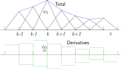
whose derivatives are bipolar "box functions"<a 
id="box_functions131698"></a>
as illustrated in Fig.&nbsp;<a href="chap13.xml#ltrianglefn">13.1</a>.

<div class="p"><!----></div>
<a id="tth_fIg13.1">
</a> <img src="figures/trianglefn.png" alt="figures/trianglefn.png" /><a id="trianglefn">
</a>

<div style="text-align:center">Figure 13.1: Localized triangle functions in one dimension, multiplied by
  coefficients, sum to a
  piecewise linear total function. Their derivatives are box functions
  with positive and negative parts. They overlap only with adjacent functions.<a id="ltrianglefn">
</a></div>

<div class="p"><!----></div>
Such a set of functions will give rise to a matrix <math xmlns="http://www.w3.org/1998/Math/MathML">
<mrow><mi mathvariant="bold">K</mi></mrow></math> that is
tridiagonal<a 
id="tridiagonal131699"></a>, just as was the case for finite
differences in one dimension. Using smoother, higher order, functions
representing the elements is sometimes advantageous. Cubic Hermite
functions, and cubic B-splines are two examples. They lead to a matrix
that is not quite as sparse, possessing typically seven non-zero
diagonals (in 1-dimension). Their ability to treat higher-order
differential equations efficiently compensates for the extra
computational complexity and cost.

<div class="p"><!----></div>
In multiple dimensions, the geometry becomes somewhat more
complicated, but, for example, there is a straightforward extension of
the piecewise linear treatment to an unstructured mesh of
tetrahedra<a 
id="tetrahedral_mesh131700"></a> 
in three dimensions. 

<div class="p"><!----></div>
<a id="tth_fIg13.2">
</a> <img src="figures/lintetrahedron.png" alt="figures/lintetrahedron.png" /><a id="lintetrahedron">
</a>
<img src="figures/tetrahedron.gif" alt="figures/tetrahedron.gif" />

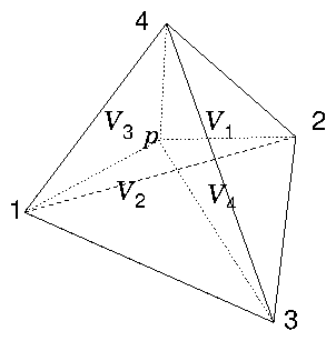
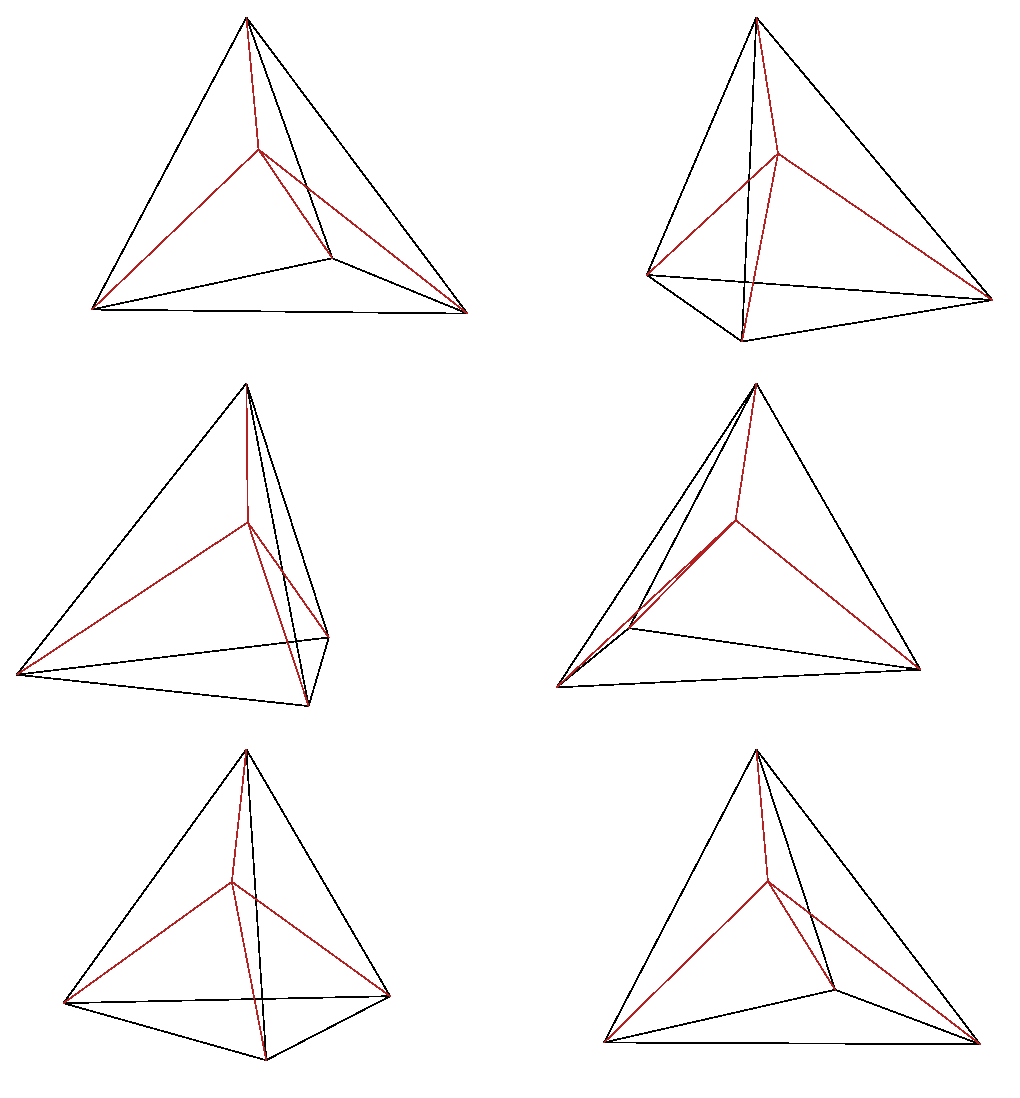
<div style="text-align:center">Figure 13.2: In linear interpolation within a tetrahedron, the lines from
  a point <math xmlns="http://www.w3.org/1998/Math/MathML">
<mrow><mi>p</mi></mrow></math> to the corner nodes of the tetrahedron, divide it into
  four smaller tetrahedra, whose volumes sum to the total volume. The
  interpolation weight of node <math xmlns="http://www.w3.org/1998/Math/MathML">
<mrow><mi>k</mi></mrow></math> is proportional to the
  corresponding volume, <math xmlns="http://www.w3.org/1998/Math/MathML">
<mrow>
<msub><mrow><mi>V</mi></mrow><mrow><mi>k</mi></mrow>
</msub>
</mrow></math>.<a id="tetral">
</a></div>

<div class="p"><!----></div>
For any point within a particular tetrahedron,
the interpolated value of the function is taken to be equal to a
weighted sum of the values at the four corner nodes. The weight of
each corner is equal to the volume of the smaller tetrahedron obtained
by replacing the corner with the point of interest, divided by the
total volume of the original tetrahedron, which Fig.&nbsp;<a href="chap13.xml#tetral">13.2</a> illustrates<a href="footnote.xml#tthFtNtAIB" id="tthFrefAIB"><math xmlns="http://www.w3.org/1998/Math/MathML">
<mrow>
<msup><mrow></mrow><mrow><mn>81</mn></mrow>
</msup>
</mrow></math></a>.  The <math xmlns="http://www.w3.org/1998/Math/MathML">
<mrow>
<msub><mrow><mi mathvariant="italic">&psi;</mi></mrow><mrow><mi>k</mi></mrow>
</msub>
</mrow></math> function associated with a node <math xmlns="http://www.w3.org/1998/Math/MathML">
<mrow><mi>k</mi></mrow></math> is unity at
that node and decreases linearly to zero along every connection leg
to an adjacent node. The
interpolation<a 
id="tetrahedral_interpolation131701"></a> formula within a single
tetrahedral element is then
<a id="interpelem">
</a><br />
<table width="100%"><tr><td align="center">
    <math xmlns="http://www.w3.org/1998/Math/MathML">
    <mstyle displaystyle="true"><mrow><mi mathvariant="italic">&psi;</mi><mo stretchy="false">(</mo><mi>p</mi><mo stretchy="false">)</mo><mo>=</mo>
<munderover><mo>&sum;</mo><mrow><mn>1</mn> </mrow>
<mrow><mn>4</mn></mrow></munderover>
<msub><mrow><mi>V</mi></mrow><mrow><mi>k</mi></mrow>
</msub>

<msub><mrow><mi>a</mi></mrow><mrow><mi>k</mi></mrow>
</msub>
<mo stretchy="false">/</mo><mi>V</mi><mo>.</mo></mrow>
    </mstyle></math></td><td width="1">
    <math xmlns="http://www.w3.org/1998/Math/MathML">
    <mstyle displaystyle="true"><mrow><mo stretchy="false">(</mo><mn>13</mn><mo>.</mo><mn>8</mn><mo stretchy="false">)</mo></mrow>
    </mstyle></math>
</td></tr></table>


In the resulting matrix <math xmlns="http://www.w3.org/1998/Math/MathML">
<mrow><mi mathvariant="bold">K</mi></mrow></math> the only non-zero overlap integrals
(coefficients) for each row <math xmlns="http://www.w3.org/1998/Math/MathML">
<mrow><mi>j</mi></mrow></math> are those for nodes <math xmlns="http://www.w3.org/1998/Math/MathML">
<mrow><mi>k</mi></mrow></math> that connect
to node <math xmlns="http://www.w3.org/1998/Math/MathML">
<mrow><mi>j</mi></mrow></math>. The number of such connections is generally small,
amounting to typically about ten per node, but depending on
the details of the mesh.  Therefore <math xmlns="http://www.w3.org/1998/Math/MathML">
<mrow><mi mathvariant="bold">K</mi></mrow></math> is very sparse; and the
necessary computational effort to obtain the solution can be greatly
reduced when advanced sparse-matrix techniques are employed. 

<div class="p"><!----></div>
More complicated meshes are also possible, using as elements other
polyhedra<a 
id="polyhedra131702"></a> such as hexahedra (non-rectangular
cubes). Also higher order interpolations of the solution within the
elements are sometimes used.  These lead to increasing complications
in handling the geometrical aspects of the problem. (Even without
these enhancements, the coding complications are already significant.)
Generally, mesh-generation libraries or applications are used to
construct the nodal mesh and its connections. Then the overlap
integrals need to be evaluated to construct the matrix <math xmlns="http://www.w3.org/1998/Math/MathML">
<mrow><mi mathvariant="bold">K</mi></mrow></math> and
the vector <math xmlns="http://www.w3.org/1998/Math/MathML">
<mrow><mi mathvariant="bold">f</mi></mrow></math>.<a href="footnote.xml#tthFtNtAIC" id="tthFrefAIC"><math xmlns="http://www.w3.org/1998/Math/MathML">
<mrow>
<msup><mrow></mrow><mrow><mn>82</mn></mrow>
</msup>
</mrow></math></a>  In
addition to open source libraries, many commercial computing packages
provide the mechanisms for mesh generation, integration, and equation
discretization, often with substantial graphical user interfaces to
ease the process.

<div class="p"><!----></div>
 <a id="tth_sEc13.2"></a><h2>
13.2&nbsp;&nbsp;Discrete Fourier Analysis and Spectral Methods</h2>

<div class="p"><!----></div>
<a 
id="Fourier_discrete_analysis132703"></a><a 
id="Fourier_methods132704"></a><a 
id="spectral_methods132705"></a>A function <math xmlns="http://www.w3.org/1998/Math/MathML">
<mrow><mi>f</mi><mo stretchy="false">(</mo><mi>t</mi><mo stretchy="false">)</mo></mrow></math>, defined over a finite range of its
argument <math xmlns="http://www.w3.org/1998/Math/MathML">
<mrow><mn>0</mn><mo>&le;</mo><mi>t</mi><mo>&lt;</mo><mi>T</mi></mrow></math> can be expressed in terms of a Fourier series
of discrete frequencies <math xmlns="http://www.w3.org/1998/Math/MathML">
<mrow>
<msub><mrow><mi mathvariant="italic">&omega;</mi></mrow><mrow><mi>n</mi></mrow>
</msub>
<mo>=</mo><mn>2</mn><mi mathvariant="italic">&pi;</mi>
<msub><mrow><mi mathvariant="italic">&nu;</mi></mrow><mrow><mi>n</mi></mrow>
</msub>
<mo>=</mo><mn>2</mn><mi mathvariant="italic">&pi;</mi><mi>n</mi><mo stretchy="false">/</mo><mi>T</mi></mrow></math> as.
<a id="FourierSeries">
</a><br />
<table width="100%"><tr><td align="center">
    <math xmlns="http://www.w3.org/1998/Math/MathML">
    <mstyle displaystyle="true"><mrow><mi>f</mi><mo stretchy="false">(</mo><mi>t</mi><mo stretchy="false">)</mo><mo>=</mo>
<munderover><mo>&sum;</mo><mrow><mi>n</mi><mo>=</mo><mo>-</mo><mi mathvariant="italic">&infin;</mi> </mrow>
<mrow><mi mathvariant="italic">&infin;</mi></mrow></munderover>
<msup><mrow><mi fontstyle="normal">e</mi></mrow><mrow><mi>i</mi>
<msub><mrow><mi mathvariant="italic">&omega;</mi></mrow><mrow><mi>n</mi></mrow>
</msub>
<mi>t</mi></mrow>
</msup>

<msub><mrow><mi>F</mi></mrow><mrow><mi>n</mi></mrow>
</msub>
<mo>,</mo></mrow>
    </mstyle></math></td><td width="1">
    <math xmlns="http://www.w3.org/1998/Math/MathML">
    <mstyle displaystyle="true"><mrow><mo stretchy="false">(</mo><mn>13</mn><mo>.</mo><mn>9</mn><mo stretchy="false">)</mo></mrow>
    </mstyle></math>
</td></tr></table>


where the Fourier coefficient for integer <math xmlns="http://www.w3.org/1998/Math/MathML">
<mrow><mi>n</mi></mrow></math> is
<a id="Fouriercoef">
</a><br />
<table width="100%"><tr><td align="center">
    <math xmlns="http://www.w3.org/1998/Math/MathML">
    <mstyle displaystyle="true"><mrow>
<msub><mrow><mi>F</mi></mrow><mrow><mi>n</mi></mrow>
</msub>
<mo>=</mo>
<mfrac><mrow><mn>1</mn></mrow>
<mrow><mi>T</mi></mrow>
</mfrac>

<msubsup><mrow><mo>&int;</mo></mrow><mrow><mn>0</mn> </mrow>
<mrow><mi>T</mi></mrow></msubsup>

<msup><mrow><mi fontstyle="normal">e</mi></mrow><mrow><mo>-</mo><mi>i</mi>
<msub><mrow><mi mathvariant="italic">&omega;</mi></mrow><mrow><mi>n</mi></mrow>
</msub>
<mi>t</mi></mrow>
</msup>
<mi>f</mi><mo stretchy="false">(</mo><mi>t</mi><mo stretchy="false">)</mo><mi mathvariant="italic">dt</mi><mo>.</mo></mrow>
    </mstyle></math></td><td width="1">
    <math xmlns="http://www.w3.org/1998/Math/MathML">
    <mstyle displaystyle="true"><mrow><mo stretchy="false">(</mo><mn>13</mn><mo>.</mo><mn>10</mn><mo stretchy="false">)</mo></mrow>
    </mstyle></math>
</td></tr></table>


Actually the expression (<a href="chap13.xml#FourierSeries">13.9</a>) gives a function <math xmlns="http://www.w3.org/1998/Math/MathML">
<mrow><mi>f</mi><mo stretchy="false">(</mo><mi>t</mi><mo stretchy="false">)</mo></mrow></math> that is
<em>periodic</em> in <math xmlns="http://www.w3.org/1998/Math/MathML">
<mrow><mi>t</mi></mrow></math> with period <math xmlns="http://www.w3.org/1998/Math/MathML">
<mrow><mi>T</mi></mrow></math>.

<div class="p"><!----></div>
Numerical representations are not usually continuous; they are
discrete. So suppose the function <math xmlns="http://www.w3.org/1998/Math/MathML">
<mrow><mi>f</mi></mrow></math> is given only at uniformly
spaced argument values <math xmlns="http://www.w3.org/1998/Math/MathML">
<mrow>
<msub><mrow><mi>t</mi></mrow><mrow><mi>j</mi></mrow>
</msub>
<mo>=</mo><mi>j</mi><mi mathvariant="italic">&Delta;</mi><mi>t</mi></mrow></math> for <math xmlns="http://www.w3.org/1998/Math/MathML">
<mrow><mi>j</mi><mo>=</mo><mn>0</mn><mo>,</mo><mn>1</mn><mo>,</mo><mo>.</mo><mo>.</mo><mo>.</mo><mo>,</mo><mi>N</mi><mo>-</mo><mn>1</mn></mrow></math>, where
<math xmlns="http://www.w3.org/1998/Math/MathML">
<mrow><mi mathvariant="italic">&Delta;</mi><mi>t</mi><mo>=</mo><mi>T</mi><mo stretchy="false">/</mo><mi>N</mi></mrow></math>, and write <math xmlns="http://www.w3.org/1998/Math/MathML">
<mrow><mi>f</mi><mo stretchy="false">(</mo>
<msub><mrow><mi>t</mi></mrow><mrow><mi>j</mi></mrow>
</msub>
<mo stretchy="false">)</mo><mo>=</mo>
<msub><mrow><mi>f</mi></mrow><mrow><mi>j</mi></mrow>
</msub>
</mrow></math>. Then these <math xmlns="http://www.w3.org/1998/Math/MathML">
<mrow><mi>N</mi></mrow></math> discrete
values<a href="footnote.xml#tthFtNtAID" id="tthFrefAID"><math xmlns="http://www.w3.org/1998/Math/MathML">
<mrow>
<msup><mrow></mrow><mrow><mn>83</mn></mrow>
</msup>
</mrow></math></a> of <math xmlns="http://www.w3.org/1998/Math/MathML">
<mrow><mi>f</mi></mrow></math> allow
us to determine only <math xmlns="http://www.w3.org/1998/Math/MathML">
<mrow><mi>N</mi></mrow></math> Fourier coefficients. It is intuitive that
these should be the <math xmlns="http://www.w3.org/1998/Math/MathML">
<mrow><mi>N</mi></mrow></math> <em>lowest</em> (absolute) frequency components,
since one clearly cannot meaningfully represent frequencies higher than
roughly <math xmlns="http://www.w3.org/1998/Math/MathML">
<mrow><mn>1</mn><mo stretchy="false">/</mo><mi mathvariant="italic">&Delta;</mi><mi>t</mi></mrow></math> on this discrete mesh. The lowest <math xmlns="http://www.w3.org/1998/Math/MathML">
<mrow><mi>N</mi></mrow></math> frequencies
are those for which <math xmlns="http://www.w3.org/1998/Math/MathML">
<mrow><mo>-</mo><mi>N</mi><mo stretchy="false">/</mo><mn>2</mn><mo>&lt;</mo><mi>n</mi><mo>&le;</mo><mi>N</mi><mo stretchy="false">/</mo><mn>2</mn></mrow></math>. This observation immediately
refines the qualification of how high a frequency can be represented
on a discrete mesh. The highest frequency<a href="footnote.xml#tthFtNtAIE" id="tthFrefAIE"><math xmlns="http://www.w3.org/1998/Math/MathML">
<mrow>
<msup><mrow></mrow><mrow><mn>84</mn></mrow>
</msup>
</mrow></math></a>  has <math xmlns="http://www.w3.org/1998/Math/MathML">
<mrow><mo stretchy="false">&verbar;</mo><mi>n</mi><mo stretchy="false">&verbar;</mo><mo>=</mo><mi>N</mi><mo stretchy="false">/</mo><mn>2</mn></mrow></math>, giving <math xmlns="http://www.w3.org/1998/Math/MathML">
<mrow>
<msub><mrow><mi mathvariant="italic">&omega;</mi></mrow><mrow><mi>n</mi></mrow>
</msub>
<mo>=</mo><mn>2</mn><mi mathvariant="italic">&pi;</mi>
<msub><mrow><mi mathvariant="italic">&nu;</mi></mrow><mrow><mi>n</mi></mrow>
</msub>
<mo>=</mo><mn>2</mn><mi mathvariant="italic">&pi;</mi><mi>N</mi><mo stretchy="false">/</mo><mn>2</mn><mi>T</mi><mo>=</mo><mi mathvariant="italic">&pi;</mi><mo stretchy="false">/</mo><mi mathvariant="italic">&Delta;</mi><mi>t</mi></mrow></math>. This limit is called the Nyquist
limit<a 
id="Nyquist_limit132706"></a>.

<div class="p"><!----></div>
If, discarding all pretence at rigor, we decide to approximate <math xmlns="http://www.w3.org/1998/Math/MathML">
<mrow><mi>f</mi></mrow></math> as
a sum of Dirac delta functions <math xmlns="http://www.w3.org/1998/Math/MathML">
<mrow><mi>f</mi><mo stretchy="false">(</mo><mi>t</mi><mo stretchy="false">)</mo><mo>&ap;</mo>
<munder><mo>&sum;</mo><mrow><mi>j</mi></mrow>
</munder>
<mi mathvariant="italic">&Delta;</mi><mi>t</mi>
<msub><mrow><mi>f</mi></mrow><mrow><mi>j</mi></mrow>
</msub>
<mi mathvariant="italic">&delta;</mi><mo stretchy="false">(</mo><mi>t</mi><mo>-</mo>
<msub><mrow><mi>t</mi></mrow><mrow><mi>j</mi></mrow>
</msub>
<mo stretchy="false">)</mo></mrow></math> (which gives approximately correct integrals), then
the integral for <math xmlns="http://www.w3.org/1998/Math/MathML">
<mrow>
<msub><mrow><mi>F</mi></mrow><mrow><mi>n</mi></mrow>
</msub>
</mrow></math> (<a href="chap13.xml#Fouriercoef">13.10</a>) can be expressed
approximately<a 
id="Fourier_transform132707"></a> as a
sum<a href="footnote.xml#tthFtNtAIF" id="tthFrefAIF"><math xmlns="http://www.w3.org/1998/Math/MathML">
<mrow>
<msup><mrow></mrow><mrow><mn>85</mn></mrow>
</msup>
</mrow></math></a>:
<a id="Fsumappr">
</a><br />
<table width="100%"><tr><td align="center">
    <math xmlns="http://www.w3.org/1998/Math/MathML">
    <mstyle displaystyle="true"><mrow>
<msub><mrow><mi>F</mi></mrow><mrow><mi>n</mi></mrow>
</msub>
<mo>=</mo>
<mfrac><mrow><mn>1</mn></mrow>
<mrow><mi>T</mi></mrow>
</mfrac>

<msubsup><mrow><mo>&int;</mo></mrow><mrow><mn>0</mn><mo>-</mo><mi mathvariant="italic">&epsi;</mi> </mrow>
<mrow><mi>T</mi><mo>-</mo><mi mathvariant="italic">&epsi;</mi></mrow></msubsup>

<msup><mrow><mi fontstyle="normal">e</mi></mrow><mrow><mo>-</mo><mi>i</mi>
<msub><mrow><mi mathvariant="italic">&omega;</mi></mrow><mrow><mi>n</mi></mrow>
</msub>
<mi>t</mi></mrow>
</msup>
<mi>f</mi><mo stretchy="false">(</mo><mi>t</mi><mo stretchy="false">)</mo><mi mathvariant="italic">dt</mi><mo>&ap;</mo>
<mfrac><mrow><mn>1</mn></mrow>
<mrow><mi>T</mi></mrow>
</mfrac>

<munderover><mo>&sum;</mo><mrow><mi>j</mi><mo>=</mo><mn>0</mn> </mrow>
<mrow><mi>N</mi><mo>-</mo><mn>1</mn></mrow></munderover>
<msup><mrow><mi fontstyle="normal">e</mi></mrow><mrow><mo>-</mo><mi>i</mi>
<msub><mrow><mi mathvariant="italic">&omega;</mi></mrow><mrow><mi>n</mi></mrow>
</msub>

<msub><mrow><mi>t</mi></mrow><mrow><mi>j</mi></mrow>
</msub>
</mrow>
</msup>

<msub><mrow><mi>f</mi></mrow><mrow><mi>j</mi></mrow>
</msub>
<mi mathvariant="italic">&Delta;</mi><mi>t</mi><mo>=</mo>
<mfrac><mrow><mn>1</mn></mrow>
<mrow><mi>N</mi></mrow>
</mfrac>

<munderover><mo>&sum;</mo><mrow><mi>j</mi><mo>=</mo><mn>0</mn> </mrow>
<mrow><mi>N</mi><mo>-</mo><mn>1</mn></mrow></munderover>
<msup><mrow><mi fontstyle="normal">e</mi></mrow><mrow><mo>-</mo><mi>i</mi><mn>2</mn><mi mathvariant="italic">&pi;</mi><mi>n</mi><mi>j</mi><mo stretchy="false">/</mo><mi>N</mi></mrow>
</msup>

<msub><mrow><mi>f</mi></mrow><mrow><mi>j</mi></mrow>
</msub>
<mo>.</mo></mrow>
    </mstyle></math></td><td width="1">
    <math xmlns="http://www.w3.org/1998/Math/MathML">
    <mstyle displaystyle="true"><mrow><mo stretchy="false">(</mo><mn>13</mn><mo>.</mo><mn>11</mn><mo stretchy="false">)</mo></mrow>
    </mstyle></math>
</td></tr></table>


Now we notice that the final expression for <math xmlns="http://www.w3.org/1998/Math/MathML">
<mrow>
<msub><mrow><mi>F</mi></mrow><mrow><mi>n</mi></mrow>
</msub>
</mrow></math> is <em>periodic</em>
with period <math xmlns="http://www.w3.org/1998/Math/MathML">
<mrow><mi>N</mi></mrow></math>; that is, <math xmlns="http://www.w3.org/1998/Math/MathML">
<mrow>
<msub><mrow><mi>F</mi></mrow><mrow><mi>n</mi><mo>+</mo><mi>N</mi></mrow>
</msub>
<mo>=</mo>
<msub><mrow><mi>F</mi></mrow><mrow><mi>n</mi></mrow>
</msub>
</mrow></math>. It is therefore convenient to
consider the range of frequency index <math xmlns="http://www.w3.org/1998/Math/MathML">
<mrow><mo>-</mo><mi>N</mi><mo stretchy="false">/</mo><mn>2</mn><mo>&lt;</mo><mi>n</mi><mo>&le;</mo><mi>N</mi><mo stretchy="false">/</mo><mn>2</mn></mrow></math> to be re-ordered
by replacing every negative <math xmlns="http://www.w3.org/1998/Math/MathML">
<mrow><mi>n</mi></mrow></math> by the positive value <math xmlns="http://www.w3.org/1998/Math/MathML">
<mrow><mi>n</mi><mo>+</mo><mi>N</mi></mrow></math>. Then <math xmlns="http://www.w3.org/1998/Math/MathML">
<mrow><mi>n</mi></mrow></math>
runs from <math xmlns="http://www.w3.org/1998/Math/MathML">
<mrow><mn>0</mn></mrow></math> to <math xmlns="http://www.w3.org/1998/Math/MathML">
<mrow><mi>N</mi><mo>-</mo><mn>1</mn></mrow></math>. One should remember, though that the upper
half of this range really represents negative
frequencies. Incidentally, the periodicity of <math xmlns="http://www.w3.org/1998/Math/MathML">
<mrow>
<msub><mrow><mi>F</mi></mrow><mrow><mi>n</mi></mrow>
</msub>
</mrow></math> illustrates that
one can equally well consider <math xmlns="http://www.w3.org/1998/Math/MathML">
<mrow>
<msub><mrow><mi>F</mi></mrow><mrow><mi>n</mi></mrow>
</msub>
</mrow></math> to represent <em>any</em> frequency
<math xmlns="http://www.w3.org/1998/Math/MathML">
<mrow><mi mathvariant="italic">&nu;</mi><mo>=</mo><mo stretchy="false">(</mo><mi>n</mi><mo>+</mo><mi mathvariant="italic">kN</mi><mo stretchy="false">)</mo><mo stretchy="false">/</mo><mi>T</mi></mrow></math> with <math xmlns="http://www.w3.org/1998/Math/MathML">
<mrow><mi>k</mi></mrow></math> an integer. That is because sampling a
continuous function <math xmlns="http://www.w3.org/1998/Math/MathML">
<mrow>
<msup><mrow><mi fontstyle="normal">e</mi></mrow><mrow><mi>i</mi><mn>2</mn><mi mathvariant="italic">&pi;</mi><mo stretchy="false">(</mo><mi>n</mi><mo>+</mo><mi mathvariant="italic">kN</mi><mo stretchy="false">)</mo><mi>t</mi><mo stretchy="false">/</mo><mi>T</mi></mrow>
</msup>
</mrow></math> at <math xmlns="http://www.w3.org/1998/Math/MathML">
<mrow><mi>t</mi><mo>=</mo><mi>j</mi><mi mathvariant="italic">&Delta;</mi><mi>t</mi><mo>=</mo><mi>j</mi><mi>T</mi><mo stretchy="false">/</mo><mi>N</mi></mrow></math>
gives values independent of <math xmlns="http://www.w3.org/1998/Math/MathML">
<mrow><mi>k</mi></mrow></math>. Thus, all frequencies higher than the
Nyquist limit <math xmlns="http://www.w3.org/1998/Math/MathML">
<mrow><mi mathvariant="italic">&nu;</mi><mo>=</mo><mi>N</mi><mo stretchy="false">/</mo><mn>2</mn><mi>T</mi></mrow></math>, contained in a continuous signal sampled
discretely, are shifted into the Nyquist range and appear at a lower
absolute frequency in the sampled representation. This effect is called aliasing<a 
id="aliasing132708"></a>.

<div class="p"><!----></div>
The <b><em>discrete</em> Fourier transform</b> and its inverse can thus be
considered to be<a 
id="Fourier_transform_discrete132709"></a>
<a id="DFT">
</a><br />
<table width="100%"><tr><td align="center">
    <math xmlns="http://www.w3.org/1998/Math/MathML">
    <mstyle displaystyle="true"><mrow>
<msub><mrow><mi>f</mi></mrow><mrow><mi>j</mi></mrow>
</msub>
<mo>=</mo>
<munderover><mo>&sum;</mo><mrow><mi>n</mi><mo>=</mo><mn>0</mn> </mrow>
<mrow><mi>N</mi><mo>-</mo><mn>1</mn></mrow></munderover>
<msup><mrow><mi fontstyle="normal">e</mi></mrow><mrow><mi>i</mi><mn>2</mn><mi mathvariant="italic">&pi;</mi><mi>n</mi><mi>j</mi><mo stretchy="false">/</mo><mi>N</mi></mrow>
</msup>

<msub><mrow><mi>F</mi></mrow><mrow><mi>n</mi></mrow>
</msub>
<mi>&ensp;</mi><mo>;</mo><mi>&emsp;&emsp;&emsp;&emsp;&emsp;&emsp;</mi>
<msub><mrow><mi>F</mi></mrow><mrow><mi>n</mi></mrow>
</msub>
<mo>=</mo>
<mfrac><mrow><mn>1</mn></mrow>
<mrow><mi>N</mi></mrow>
</mfrac>

<munderover><mo>&sum;</mo><mrow><mi>j</mi><mo>=</mo><mn>0</mn> </mrow>
<mrow><mi>N</mi><mo>-</mo><mn>1</mn></mrow></munderover>
<msup><mrow><mi fontstyle="normal">e</mi></mrow><mrow><mo>-</mo><mi>i</mi><mn>2</mn><mi mathvariant="italic">&pi;</mi><mi>n</mi><mi>j</mi><mo stretchy="false">/</mo><mi>N</mi></mrow>
</msup>

<msub><mrow><mi>f</mi></mrow><mrow><mi>j</mi></mrow>
</msub>
<mo>.</mo></mrow>
    </mstyle></math></td><td width="1">
    <math xmlns="http://www.w3.org/1998/Math/MathML">
    <mstyle displaystyle="true"><mrow><mo stretchy="false">(</mo><mn>13</mn><mo>.</mo><mn>12</mn><mo stretchy="false">)</mo></mrow>
    </mstyle></math>
</td></tr></table>


Substituting for <math xmlns="http://www.w3.org/1998/Math/MathML">
<mrow>
<msub><mrow><mi>F</mi></mrow><mrow><mi>n</mi></mrow>
</msub>
</mrow></math> in this expression for <math xmlns="http://www.w3.org/1998/Math/MathML">
<mrow>
<msub><mrow><mi>f</mi></mrow><mrow><mi>j</mi></mrow>
</msub>
</mrow></math>, one obtains
coefficients that are sums of the form <math xmlns="http://www.w3.org/1998/Math/MathML">
<mrow>
<munder><mo>&sum;</mo><mrow><mi>n</mi></mrow>
</munder>

<msup><mrow><mi fontstyle="normal">e</mi></mrow><mrow><mi>i</mi><mn>2</mn><mi mathvariant="italic">&pi;</mi><mi>n</mi><mi>j</mi><mo stretchy="false">/</mo><mi>N</mi></mrow>
</msup>

<msup><mrow><mi fontstyle="normal">e</mi></mrow><mrow><mo>-</mo><mi>i</mi><mn>2</mn><mi mathvariant="italic">&pi;</mi><mi>n</mi><mi>j</mi><mo>'</mo><mo stretchy="false">/</mo><mi>N</mi></mrow>
</msup>
</mrow></math> which is zero if <math xmlns="http://www.w3.org/1998/Math/MathML">
<mrow><mi>j</mi><mo>&ne;</mo><mi>j</mi><mo>'</mo></mrow></math> and <math xmlns="http://www.w3.org/1998/Math/MathML">
<mrow><mi>N</mi></mrow></math> if
<math xmlns="http://www.w3.org/1998/Math/MathML">
<mrow><mi>j</mi><mo>=</mo><mi>j</mi><mo>'</mo></mrow></math>. Therefore these two equations are exact, and could have been
simply adopted as definitions from the start. The discrete Fourier
transforms need not be considered <em>approximations</em> to continuous
transforms; but it is helpful to recognize their relationship to
Fourier series representations of continuous functions.

<div class="p"><!----></div>
Of course we aren't really interested in quantities that consist of a
set of delta functions. If, instead of simply multiplying by <math xmlns="http://www.w3.org/1998/Math/MathML">
<mrow><mi mathvariant="italic">&Delta;</mi><mi>t</mi></mrow></math>, we convolve <math xmlns="http://www.w3.org/1998/Math/MathML">
<mrow>
<munder><mo>&sum;</mo><mrow><mi>j</mi></mrow>
</munder>

<msub><mrow><mi>f</mi></mrow><mrow><mi>j</mi></mrow>
</msub>
<mi mathvariant="italic">&delta;</mi><mo stretchy="false">(</mo><mi>t</mi><mo>-</mo>
<msub><mrow><mi>t</mi></mrow><mrow><mi>j</mi></mrow>
</msub>
<mo stretchy="false">)</mo></mrow></math> with a triangle function
that is unity at <math xmlns="http://www.w3.org/1998/Math/MathML">
<mrow><mi>t</mi><mo>=</mo><mn>0</mn></mrow></math> and descends linearly to zero at <math xmlns="http://www.w3.org/1998/Math/MathML">
<mrow><mi>t</mi><mo>=</mo><mo>&PlusMinus;</mo><mi mathvariant="italic">&Delta;</mi><mi>t</mi></mrow></math>,
then we will recover a piecewise linear function whose values at <math xmlns="http://www.w3.org/1998/Math/MathML">
<mrow>
<msub><mrow><mi>t</mi></mrow><mrow><mi>j</mi></mrow>
</msub>
</mrow></math>
are <math xmlns="http://www.w3.org/1998/Math/MathML">
<mrow>
<msub><mrow><mi>f</mi></mrow><mrow><mi>j</mi></mrow>
</msub>
</mrow></math>. This is a much closer representation of the sort of
function we might be considering. 

<div class="p"><!----></div>
The Fourier transform of a
convolution of two functions is the product of their Fourier
transforms. 
<a id="convolu">
</a><br />
<table width="100%"><tr><td align="center">
    <math xmlns="http://www.w3.org/1998/Math/MathML">
    <mstyle displaystyle="true"><mrow>
<msubsup><mrow><mo>&int;</mo></mrow><mrow><mn>0</mn> </mrow>
<mrow><mi>T</mi></mrow></msubsup>

<msup><mrow><mi fontstyle="normal">e</mi></mrow><mrow><mo>-</mo>
<msub><mrow><mi mathvariant="italic">&omega;</mi></mrow><mrow><mi>n</mi></mrow>
</msub>
<mi>t</mi></mrow>
</msup>

<msubsup><mrow><mo>&int;</mo></mrow><mrow><mn>0</mn> </mrow>
<mrow><mi>T</mi></mrow></msubsup>
<mi>f</mi><mo stretchy="false">(</mo><mi>t</mi><mo>'</mo><mo stretchy="false">)</mo><mi>g</mi><mo stretchy="false">(</mo><mi>t</mi><mo>-</mo><mi>t</mi><mo>'</mo><mo stretchy="false">)</mo><mi mathvariant="italic">dt</mi><mo>'</mo><mi mathvariant="italic">dt</mi><mo>=</mo>
<msubsup><mrow><mo>&int;</mo></mrow><mrow><mn>0</mn> </mrow>
<mrow><mi>T</mi></mrow></msubsup>

<msup><mrow><mi fontstyle="normal">e</mi></mrow><mrow><mo>-</mo>
<msub><mrow><mi mathvariant="italic">&omega;</mi></mrow><mrow><mi>n</mi></mrow>
</msub>
<mi>t</mi><mo>'</mo></mrow>
</msup>
<mi>f</mi><mo stretchy="false">(</mo><mi>t</mi><mo>'</mo><mo stretchy="false">)</mo><mi mathvariant="italic">dt</mi><mo>'</mo>
<msubsup><mrow><mo>&int;</mo></mrow><mrow><mn>0</mn> </mrow>
<mrow><mi>T</mi></mrow></msubsup>

<msup><mrow><mi fontstyle="normal">e</mi></mrow><mrow><mo>-</mo>
<msub><mrow><mi mathvariant="italic">&omega;</mi></mrow><mrow><mi>n</mi></mrow>
</msub>
<mi>t</mi>"</mrow>
</msup>
<mi>g</mi><mo stretchy="false">(</mo><mi>t</mi>"<mo stretchy="false">)</mo><mi mathvariant="italic">dt</mi>"<mo>.</mo></mrow>
    </mstyle></math></td><td width="1">
    <math xmlns="http://www.w3.org/1998/Math/MathML">
    <mstyle displaystyle="true"><mrow><mo stretchy="false">(</mo><mn>13</mn><mo>.</mo><mn>13</mn><mo stretchy="false">)</mo></mrow>
    </mstyle></math>
</td></tr></table>


Therefore the Fourier coefficients <math xmlns="http://www.w3.org/1998/Math/MathML">
<mrow>
<msub><mrow><mi>F</mi></mrow><mrow><mi>n</mi></mrow>
</msub>
</mrow></math> corresponding to
the piecewise linear form of <math xmlns="http://www.w3.org/1998/Math/MathML">
<mrow><mi>f</mi></mrow></math> are the expressions in eq.&nbsp;(<a href="chap13.xml#DFT">13.12</a>)
multiplied by the scaled Fourier transform of the triangle function, namely
<a id="trianglFT">
</a><br />
<table width="100%"><tr><td align="center">
    <math xmlns="http://www.w3.org/1998/Math/MathML">
    <mstyle displaystyle="true"><mrow>
<msub><mrow><mi>K</mi></mrow><mrow><mi>n</mi></mrow>
</msub>
<mo>=</mo>
<msubsup><mrow><mo>&int;</mo></mrow><mrow><mo>-</mo><mi mathvariant="italic">&Delta;</mi><mi>t</mi> </mrow>
<mrow><mi mathvariant="italic">&Delta;</mi><mi>t</mi></mrow></msubsup>

<msup><mrow><mi fontstyle="normal">e</mi></mrow><mrow><mo>-</mo><mi>i</mi>
<msub><mrow><mi mathvariant="italic">&omega;</mi></mrow><mrow><mi>n</mi></mrow>
</msub>
<mi>t</mi></mrow>
</msup>
<mo stretchy="false">(</mo><mn>1</mn><mo>-</mo><mo stretchy="false">&verbar;</mo><mi>t</mi><mo stretchy="false">&verbar;</mo><mo stretchy="false">/</mo><mi mathvariant="italic">&Delta;</mi><mi>t</mi><mo stretchy="false">)</mo><mi mathvariant="italic">dt</mi><mo stretchy="false">/</mo><mi mathvariant="italic">&Delta;</mi><mi>t</mi><mo>=</mo>
<mfrac><mrow>
<msup><mrow><mi>sin</mi></mrow><mrow><mn>2</mn></mrow>
</msup>
<mo stretchy="false">(</mo>
<msub><mrow><mi mathvariant="italic">&omega;</mi></mrow><mrow><mi>n</mi></mrow>
</msub>
<mi mathvariant="italic">&Delta;</mi><mi>t</mi><mo stretchy="false">/</mo><mn>2</mn><mo stretchy="false">)</mo></mrow>
<mrow><mo stretchy="false">(</mo>
<msub><mrow><mi mathvariant="italic">&omega;</mi></mrow><mrow><mi>n</mi></mrow>
</msub>
<mi mathvariant="italic">&Delta;</mi><mi>t</mi><mo stretchy="false">/</mo><mn>2</mn>
<msup><mrow><mo stretchy="false">)</mo></mrow><mrow><mn>2</mn></mrow>
</msup>
</mrow>
</mfrac>
<mo>.</mo></mrow>
    </mstyle></math></td><td width="1">
    <math xmlns="http://www.w3.org/1998/Math/MathML">
    <mstyle displaystyle="true"><mrow><mo stretchy="false">(</mo><mn>13</mn><mo>.</mo><mn>14</mn><mo stretchy="false">)</mo></mrow>
    </mstyle></math>
</td></tr></table>


So when dealing with continuous functions, and interpolating using the
inverse transform, eq.&nbsp;(<a href="chap13.xml#FourierSeries">13.9</a>), one ought probably to filter the
signal in frequency space. Multiplying by the sinc-squared function
<math xmlns="http://www.w3.org/1998/Math/MathML">
<mrow>
<msub><mrow><mi>K</mi></mrow><mrow><mi>n</mi></mrow>
</msub>
<mo>=</mo>
<msup><mrow><mi>sin</mi></mrow><mrow><mn>2</mn></mrow>
</msup>
<mo stretchy="false">(</mo>
<msub><mrow><mi>z</mi></mrow><mrow><mi>n</mi></mrow>
</msub>
<mo stretchy="false">)</mo><mo stretchy="false">/</mo>
<msubsup><mrow><mi>z</mi></mrow><mrow><mi>n</mi> </mrow>
<mrow><mn>2</mn></mrow></msubsup>
</mrow></math>, with <math xmlns="http://www.w3.org/1998/Math/MathML">
<mrow>
<msub><mrow><mi>z</mi></mrow><mrow><mi>n</mi></mrow>
</msub>
<mo>=</mo>
<msub><mrow><mi mathvariant="italic">&omega;</mi></mrow><mrow><mi>n</mi></mrow>
</msub>
<mi mathvariant="italic">&Delta;</mi><mi>t</mi><mo stretchy="false">/</mo><mn>2</mn></mrow></math> is the
equivalent of doing piecewise linear interpolation. At the highest
absolute frequency, <math xmlns="http://www.w3.org/1998/Math/MathML">
<mrow>
<msub><mrow><mi mathvariant="italic">&omega;</mi></mrow><mrow><mi>N</mi><mo stretchy="false">/</mo><mn>2</mn></mrow>
</msub>
</mrow></math>, where <math xmlns="http://www.w3.org/1998/Math/MathML">
<mrow>
<msub><mrow><mi mathvariant="italic">&omega;</mi></mrow><mrow><mi>n</mi></mrow>
</msub>
<mi mathvariant="italic">&Delta;</mi><mi>t</mi><mo stretchy="false">/</mo><mn>2</mn><mo>=</mo><mi mathvariant="italic">&pi;</mi><mi>N</mi><mi mathvariant="italic">&Delta;</mi><mi>T</mi><mo stretchy="false">/</mo><mi>T</mi><mo>=</mo><mi mathvariant="italic">&pi;</mi></mrow></math>, the filter reaches its first zero. It modestly
 limits the frequency bandwidth of the signal.

<div class="p"><!----></div>
 It turns out to be possible to evaluate discrete Fourier transforms
 (by successively dividing the domain in half) much faster than
 implementing the <math xmlns="http://www.w3.org/1998/Math/MathML">
<mrow><mi>N</mi><mo>&times;</mo><mi>N</mi></mrow></math> multiplications implied by performing
 the sums in eq.&nbsp;(<a href="chap13.xml#DFT">13.12</a>) one after the other. The
 algorithms<a 
id="Fourier_transform_fast132710"></a><a 
id="fast_Fourier____transform132711"></a> that reduce the computational effort to of order <math xmlns="http://www.w3.org/1998/Math/MathML">
<mrow><mi>N</mi><mi>ln</mi><mi>N</mi></mrow></math> multiplications are called Fast Fourier Transforms<a href="footnote.xml#tthFtNtAIG" id="tthFrefAIG"><math xmlns="http://www.w3.org/1998/Math/MathML">
<mrow>
<msup><mrow></mrow><mrow><mn>86</mn></mrow>
</msup>
</mrow></math></a>. They, naturally enough, find important uses in
 spectral analysis and filtering. But, less obviously, they also
 provide powerful techniques for solving partial differential
 equations by representing the solution in terms of a finite number of
 Fourier coeffients, as an alternative to a finite number of discrete
 values.

<div class="p"><!----></div>
 <b>Spectral representation</b><a 
id="spectral_representation132712"></a> is
 most powerful for linear problems in which there is an ignorable
 coordinate<a 
id="ignorable_coordinate132713"></a> because of some inherent
 symmetry. In such situations each Fourier component becomes
 independent of the others. What's more, the Fourier components are
 the eigenmodes (in the direction of symmetry) of the
 problem. Consequently it is sometimes the case that including a very
 few such Fourier components, even as few as one, can represent the
 solution. In effect, this practically lowers the dimensionality of
 the problem by one, leading to major computational advantage. The
 equations can be formulated in terms of Fourier modes in the symmetry
 direction and finite differences in the other direction(s). For
 separable<a 
id="separable_coordinates132714"></a> linear problems like this,
 there is actually no pressing need for the Fourier Transforms to be
 <em>Fast</em>, because the solution in space only needs to be
 reconstructed after the solution in terms of Fourier modes has been
 found.

<div class="p"><!----></div>
If the equations to be solved are non-linear, however, or the symmetry is only
approximate, then different Fourier modes are coupled together. Then a
larger number of modes is necessary, and the computational advantage
becomes less. Even so, there are sometimes substantial remaining
benefits to a spectral representation, provided the Fourier transform
is fast. The advantages can be understood as follows. 

<div class="p"><!----></div>
Suppose we have a partial differential equation in which we wish to
represent the <math xmlns="http://www.w3.org/1998/Math/MathML">
<mrow><mi>x</mi></mrow></math> coordinate by a Fourier expansion. The
representations of the other coordinates and their differentials do
not affect this question. Consider the equation to consist of a part
that is linear in the dependent variable <math xmlns="http://www.w3.org/1998/Math/MathML">
<mrow><mi>u</mi></mrow></math>, <math xmlns="http://www.w3.org/1998/Math/MathML">
<mrow><mrow><mstyle fontfamily="helvetica"><mi fontstyle="italic">L</mi></mstyle></mrow>
<mo stretchy="false">(</mo><mi>u</mi><mo stretchy="false">)</mo></mrow></math> and a part
that is quadratic <math xmlns="http://www.w3.org/1998/Math/MathML">
<mrow><mrow><mstyle fontfamily="helvetica"><mi fontstyle="italic">M</mi></mstyle></mrow>
<mo stretchy="false">(</mo><mi>u</mi><mo stretchy="false">)</mo><mrow><mstyle fontfamily="helvetica"><mi fontstyle="italic">N</mi></mstyle></mrow>
<mo stretchy="false">(</mo><mi>u</mi><mo stretchy="false">)</mo></mrow></math><a 
id="non-linearity132715"></a>; so
<br />
<table width="100%"><tr><td align="center">
    <math xmlns="http://www.w3.org/1998/Math/MathML">
    <mstyle displaystyle="true"><mrow><mrow><mstyle fontfamily="helvetica"><mi fontstyle="italic">L</mi></mstyle></mrow>
<mo stretchy="false">(</mo><mi>u</mi><mo stretchy="false">)</mo><mo>+</mo><mrow><mstyle fontfamily="helvetica"><mi fontstyle="italic">M</mi></mstyle></mrow>
<mo stretchy="false">(</mo><mi>u</mi><mo stretchy="false">)</mo><mrow><mstyle fontfamily="helvetica"><mi fontstyle="italic">N</mi></mstyle></mrow>
<mo stretchy="false">(</mo><mi>u</mi><mo stretchy="false">)</mo><mo>=</mo><mi>s</mi><mo stretchy="false">(</mo><mi>x</mi><mo stretchy="false">)</mo><mo>.</mo></mrow>
    </mstyle></math></td><td width="1">
    <math xmlns="http://www.w3.org/1998/Math/MathML">
    <mstyle displaystyle="true"><mrow><mo stretchy="false">(</mo><mn>13</mn><mo>.</mo><mn>15</mn><mo stretchy="false">)</mo></mrow>
    </mstyle></math>
</td></tr></table>


Here <math xmlns="http://www.w3.org/1998/Math/MathML">
<mrow><mrow><mstyle fontfamily="helvetica"><mi fontstyle="italic">L</mi></mstyle></mrow>
</mrow></math>, <math xmlns="http://www.w3.org/1998/Math/MathML">
<mrow><mrow><mstyle fontfamily="helvetica"><mi fontstyle="italic">M</mi></mstyle></mrow>
</mrow></math>, <math xmlns="http://www.w3.org/1998/Math/MathML">
<mrow><mrow><mstyle fontfamily="helvetica"><mi fontstyle="italic">N</mi></mstyle></mrow>
</mrow></math> are linear <math xmlns="http://www.w3.org/1998/Math/MathML">
<mrow><mi>x</mi></mrow></math>-differential
operators, for example: <math xmlns="http://www.w3.org/1998/Math/MathML">
<mrow><mrow><mstyle fontfamily="helvetica"><mi fontstyle="italic">L</mi></mstyle></mrow>
<mo stretchy="false">(</mo><mi>u</mi><mo stretchy="false">)</mo><mo>=</mo>
<mfrac><mrow><mo>&part;</mo><mi>u</mi></mrow>
<mrow><mo>&part;</mo><mi>x</mi></mrow>
</mfrac>
<mo>+</mo><mi>g</mi><mi>u</mi></mrow></math>. We represent <math xmlns="http://www.w3.org/1998/Math/MathML">
<mrow><mi>u</mi></mrow></math> by a sum of <math xmlns="http://www.w3.org/1998/Math/MathML">
<mrow><mi>N</mi></mrow></math> Fourier modes <math xmlns="http://www.w3.org/1998/Math/MathML">
<mrow><mi>u</mi><mo>=</mo>
<munderover><mo>&sum;</mo><mrow><mi>n</mi><mo>=</mo><mn>1</mn> </mrow>
<mrow><mi>N</mi></mrow></munderover>
<msup><mrow><mi fontstyle="normal">e</mi></mrow><mrow>
<msub><mrow><mi mathvariant="italic">ik</mi></mrow><mrow><mi>n</mi></mrow>
</msub>
<mi>x</mi></mrow>
</msup>

<msub><mrow><mi>U</mi></mrow><mrow><mi>n</mi></mrow>
</msub>
</mrow></math>, where for an <math xmlns="http://www.w3.org/1998/Math/MathML">
<mrow><mi>x</mi></mrow></math>-domain of length <math xmlns="http://www.w3.org/1998/Math/MathML">
<mrow><mi>X</mi></mrow></math>, <math xmlns="http://www.w3.org/1998/Math/MathML">
<mrow>
<msub><mrow><mi>k</mi></mrow><mrow><mi>n</mi></mrow>
</msub>
<mo>=</mo><mn>2</mn><mi mathvariant="italic">&pi;</mi><mi>n</mi><mo stretchy="false">/</mo><mi>X</mi></mrow></math>. Substituting a Fourier mode into a linear operator gives rise
to an algebraic multiplier. For example <math xmlns="http://www.w3.org/1998/Math/MathML">
<mrow><mrow><mo>(</mo>
<mfrac><mrow><mo>&part;</mo></mrow>
<mrow><mo>&part;</mo><mi>x</mi></mrow>
</mfrac>
<mo>+</mo><mi>g</mi><mo>)</mo></mrow>
<msup><mrow><mi fontstyle="normal">e</mi></mrow><mrow>
<msub><mrow><mi mathvariant="italic">ik</mi></mrow><mrow><mi>n</mi></mrow>
</msub>
<mi>x</mi></mrow>
</msup>
<mo>=</mo><mo stretchy="false">(</mo><mi mathvariant="italic">ik</mi><mo>+</mo><mi>g</mi><mo stretchy="false">)</mo>
<msup><mrow><mi fontstyle="normal">e</mi></mrow><mrow>
<msub><mrow><mi mathvariant="italic">ik</mi></mrow><mrow><mi>n</mi></mrow>
</msub>
<mi>x</mi></mrow>
</msup>
</mrow></math>. So <math xmlns="http://www.w3.org/1998/Math/MathML">
<mrow><mrow><mstyle fontfamily="helvetica"><mi fontstyle="italic">L</mi></mstyle></mrow>
<mo stretchy="false">(</mo><mi>u</mi><mo stretchy="false">)</mo><mo>=</mo>
<munder><mo>&sum;</mo><mrow><mi>n</mi></mrow>
</munder>

<msub><mrow><mi>L</mi></mrow><mrow><mi>n</mi></mrow>
</msub>

<msup><mrow><mi fontstyle="normal">e</mi></mrow><mrow>
<msub><mrow><mi mathvariant="italic">ik</mi></mrow><mrow><mi>n</mi></mrow>
</msub>
<mi>x</mi></mrow>
</msup>
</mrow></math>, where
<math xmlns="http://www.w3.org/1998/Math/MathML">
<mrow>
<msub><mrow><mi>L</mi></mrow><mrow><mi>n</mi></mrow>
</msub>
</mrow></math> is the multiplier arising from <math xmlns="http://www.w3.org/1998/Math/MathML">
<mrow><mrow><mstyle fontfamily="helvetica"><mi fontstyle="italic">L</mi></mstyle></mrow>
</mrow></math> for the <math xmlns="http://www.w3.org/1998/Math/MathML">
<mrow>
<msub><mrow><mi>k</mi></mrow><mrow><mi>n</mi></mrow>
</msub>
</mrow></math>
mode. The equations that determine the <math xmlns="http://www.w3.org/1998/Math/MathML">
<mrow>
<msub><mrow><mi>U</mi></mrow><mrow><mi>n</mi></mrow>
</msub>
</mrow></math> are found by Fourier
transforming the differential equation we started with:
<a id="nonlinFourier">
</a><br />
<table width="100%"><tr><td align="center">
    <math xmlns="http://www.w3.org/1998/Math/MathML">
    <mstyle displaystyle="true"><mrow>
<mfrac><mrow><mn>1</mn></mrow>
<mrow><mi>X</mi></mrow>
</mfrac>

<msubsup><mrow><mo>&int;</mo></mrow><mrow><mn>0</mn> </mrow>
<mrow><mi>X</mi></mrow></msubsup>
<mo stretchy="false">[</mo><mrow><mstyle fontfamily="helvetica"><mi fontstyle="italic">L</mi></mstyle></mrow>
<mo stretchy="false">(</mo><mi>u</mi><mo stretchy="false">)</mo><mo>+</mo><mrow><mstyle fontfamily="helvetica"><mi fontstyle="italic">M</mi></mstyle></mrow>
<mo stretchy="false">(</mo><mi>u</mi><mo stretchy="false">)</mo><mrow><mstyle fontfamily="helvetica"><mi fontstyle="italic">N</mi></mstyle></mrow>
<mo stretchy="false">(</mo><mi>u</mi><mo stretchy="false">)</mo><mo stretchy="false">]</mo>
<msup><mrow><mi fontstyle="normal">e</mi></mrow><mrow><mo>-</mo>
<msub><mrow><mi mathvariant="italic">ik</mi></mrow><mrow><mi>m</mi></mrow>
</msub>
<mi>x</mi></mrow>
</msup>
<mi mathvariant="italic">dx</mi><mo>=</mo>
<msub><mrow><mi>S</mi></mrow><mrow><mi>m</mi></mrow>
</msub>
<mo>.</mo></mrow>
    </mstyle></math></td><td width="1">
    <math xmlns="http://www.w3.org/1998/Math/MathML">
    <mstyle displaystyle="true"><mrow><mo stretchy="false">(</mo><mn>13</mn><mo>.</mo><mn>16</mn><mo stretchy="false">)</mo></mrow>
    </mstyle></math>
</td></tr></table>


Substituting in the Fourier expansion of <math xmlns="http://www.w3.org/1998/Math/MathML">
<mrow><mi>u</mi></mrow></math>, and using the orthonormal
properties of the modes: <math xmlns="http://www.w3.org/1998/Math/MathML">
<mrow>
<msubsup><mrow><mo>&int;</mo></mrow><mrow><mn>0</mn> </mrow>
<mrow><mi>X</mi></mrow></msubsup>

<msup><mrow><mi fontstyle="normal">e</mi></mrow><mrow>
<msub><mrow><mi mathvariant="italic">ik</mi></mrow><mrow><mi>n</mi></mrow>
</msub>
<mi>x</mi></mrow>
</msup>

<msup><mrow><mi fontstyle="normal">e</mi></mrow><mrow><mo>-</mo>
<msub><mrow><mi mathvariant="italic">ik</mi></mrow><mrow><mi>m</mi></mrow>
</msub>
<mi>x</mi></mrow>
</msup>
<mi mathvariant="italic">dx</mi><mo stretchy="false">/</mo><mi>X</mi><mo>=</mo>
<msub><mrow><mi mathvariant="italic">&delta;</mi></mrow><mrow><mi mathvariant="italic">mn</mi></mrow>
</msub>
</mrow></math> we get 
 <a id="prodconv">
</a><br />
<table width="100%"><tr><td align="center">
    <math xmlns="http://www.w3.org/1998/Math/MathML">
    <mstyle displaystyle="true"><mrow>
<msub><mrow><mi>L</mi></mrow><mrow><mi>m</mi></mrow>
</msub>

<msub><mrow><mi>U</mi></mrow><mrow><mi>m</mi></mrow>
</msub>

<msup><mrow><mi fontstyle="normal">e</mi></mrow><mrow>
<msub><mrow><mi mathvariant="italic">ik</mi></mrow><mrow><mi>m</mi></mrow>
</msub>
<mi>x</mi></mrow>
</msup>
<mo>+</mo>
<munder><mo>&sum;</mo><mrow><mi>l</mi><mo>+</mo><mi>n</mi><mo>=</mo><mi>m</mi></mrow>
</munder>

<msub><mrow><mi>M</mi></mrow><mrow><mi>l</mi></mrow>
</msub>

<msub><mrow><mi>U</mi></mrow><mrow><mi>l</mi></mrow>
</msub>

<msup><mrow><mi fontstyle="normal">e</mi></mrow><mrow>
<msub><mrow><mi mathvariant="italic">ik</mi></mrow><mrow><mi>l</mi></mrow>
</msub>
<mi>x</mi></mrow>
</msup>

<msub><mrow><mi>N</mi></mrow><mrow><mi>n</mi></mrow>
</msub>

<msub><mrow><mi>U</mi></mrow><mrow><mi>n</mi></mrow>
</msub>

<msup><mrow><mi fontstyle="normal">e</mi></mrow><mrow>
<msub><mrow><mi mathvariant="italic">ik</mi></mrow><mrow><mi>n</mi></mrow>
</msub>
<mi>x</mi></mrow>
</msup>
<mo>=</mo>
<msub><mrow><mi>S</mi></mrow><mrow><mi>m</mi></mrow>
</msub>
</mrow>
    </mstyle></math></td><td width="1">
    <math xmlns="http://www.w3.org/1998/Math/MathML">
    <mstyle displaystyle="true"><mrow><mo stretchy="false">(</mo><mn>13</mn><mo>.</mo><mn>17</mn><mo stretchy="false">)</mo></mrow>
    </mstyle></math>
</td></tr></table>


The sum arising from the quadratic term couples all the individual
modal equations<a 
id="coupled_equations132716"></a> together. Without it they
would be uncoupled. The coupling term has the form of a convolution
sum. To evaluate the sum directly requires for each equation <math xmlns="http://www.w3.org/1998/Math/MathML">
<mrow><mi>m</mi></mrow></math> that
we evaluate on average <math xmlns="http://www.w3.org/1998/Math/MathML">
<mrow><mi>N</mi><mo stretchy="false">/</mo><mn>2</mn></mrow></math> terms, for a total computational
multiplication count of approximately <math xmlns="http://www.w3.org/1998/Math/MathML">
<mrow><mn>2</mn>
<msup><mrow><mi>N</mi></mrow><mrow><mn>2</mn></mrow>
</msup>
</mrow></math> (because there are four
multiplications per term) per solution step. Generally a nonlinear
equation must be solved by iterative steps in which the nonlinear term
must be evaluated. An alternative way to evaluate the nonlinear term
at each step is to transform back to <math xmlns="http://www.w3.org/1998/Math/MathML">
<mrow><mi>x</mi></mrow></math>-space, perform the
multiplication on the <math xmlns="http://www.w3.org/1998/Math/MathML">
<mrow><mi>x</mi></mrow></math>-space <math xmlns="http://www.w3.org/1998/Math/MathML">
<mrow><mrow><mstyle fontfamily="helvetica"><mi fontstyle="italic">M</mi></mstyle></mrow>
<mo stretchy="false">(</mo><mi>u</mi><mo stretchy="false">)</mo><mrow><mstyle fontfamily="helvetica"><mi fontstyle="italic">N</mi></mstyle></mrow>
<mo stretchy="false">(</mo><mi>u</mi><mo stretchy="false">)</mo></mrow></math>, and then
fast Fourier transform (FFT) <a 
id="fast_Fourier_transform132717"></a>the product
again to obtain the sum term for the Fourier mode equation
(<a href="chap13.xml#prodconv">13.17</a>).  
The differencing to evaluate the operators <math xmlns="http://www.w3.org/1998/Math/MathML">
<mrow><mrow><mstyle fontfamily="helvetica"><mi fontstyle="italic">M</mi></mstyle></mrow>
</mrow></math> and <math xmlns="http://www.w3.org/1998/Math/MathML">
<mrow><mrow><mstyle fontfamily="helvetica"><mi fontstyle="italic">N</mi></mstyle></mrow>
</mrow></math>
costs a few multiplications, say <math xmlns="http://www.w3.org/1998/Math/MathML">
<mrow><mi>p</mi></mrow></math>. The product for all <math xmlns="http://www.w3.org/1998/Math/MathML">
<mrow><mi>N</mi></mrow></math> values
<math xmlns="http://www.w3.org/1998/Math/MathML">
<mrow><mi>u</mi></mrow></math> will then cost <math xmlns="http://www.w3.org/1998/Math/MathML">
<mrow><mi mathvariant="italic">Np</mi></mrow></math>. And the two FFTs will be only approximately <math xmlns="http://www.w3.org/1998/Math/MathML">
<mrow><mn>2</mn><mi>N</mi><mi>ln</mi><mi>N</mi></mrow></math>. Therefore the total cost of this alternative scales like <math xmlns="http://www.w3.org/1998/Math/MathML">
<mrow><mi>N</mi><mo stretchy="false">(</mo><mn>2</mn><mi>ln</mi><mi>N</mi><mo>+</mo><mi>p</mi><mo stretchy="false">)</mo></mrow></math>.  Thus, using the FFT approach reduces the <math xmlns="http://www.w3.org/1998/Math/MathML">
<mrow><mn>2</mn>
<msup><mrow><mi>N</mi></mrow><mrow><mn>2</mn></mrow>
</msup>
</mrow></math>
computational cost scaling to <math xmlns="http://www.w3.org/1998/Math/MathML">
<mrow><mi>N</mi><mo stretchy="false">(</mo><mn>2</mn><mi>ln</mi><mi>N</mi><mo>+</mo><mi>p</mi><mo stretchy="false">)</mo></mrow></math>.

<div class="p"><!----></div>
Some extra questions arise concerning aliasing, but
this FFT approach is nevertheless used to good advantage for some
applications. 

<div class="p"><!----></div>
 <a id="tth_sEc13.3"></a><h2>
13.3&nbsp;&nbsp;Sparse Matrix Iterative Krylov Solution</h2>

<div class="p"><!----></div>
<a 
id="Krylov_techniques133718"></a> We stopped our development of iterative
linear system solution, which we saw in Chapter <a href="chap6.xml#ChapEllip">6</a> is at
the heart of solving most boundary-value differential equations,
before introducing the most significant modern developments in this
field. These are associated with the name of Krylov. Here we give the
barest introduction. A modern text book should be consulted for more
details. First, as far as terminology is concerned, the name refers to
the use of the <em>subspace</em><a 
id="subspace_Krylov133719"></a> of a vector
space that is accessed by repeated multiplications by the same
matrix. The Krylov subspace <math xmlns="http://www.w3.org/1998/Math/MathML">
<mrow>
<msub><mrow><mstyle fontfamily="helvetica"><mi fontstyle="italic">K</mi></mstyle></mrow>
<mrow><mi>k</mi></mrow>
</msub>
<mo stretchy="false">(</mo><mi mathvariant="bold">A</mi><mo>,</mo><mi mathvariant="bold">b</mi><mo stretchy="false">)</mo></mrow></math> of dimension
<math xmlns="http://www.w3.org/1998/Math/MathML">
<mrow><mi>k</mi></mrow></math> generated by a matrix <math xmlns="http://www.w3.org/1998/Math/MathML">
<mrow><mi mathvariant="bold">A</mi></mrow></math> from an initial vector <math xmlns="http://www.w3.org/1998/Math/MathML">
<mrow><mi mathvariant="bold">b</mi></mrow></math>
consists of all vectors that can be expressed in the form of a sum of
coefficients times the vectors <math xmlns="http://www.w3.org/1998/Math/MathML">
<mrow>
<msup><mrow><mi mathvariant="bold">A</mi></mrow><mrow><mi>j</mi></mrow>
</msup>
<mi mathvariant="bold">b</mi></mrow></math>, for <math xmlns="http://www.w3.org/1998/Math/MathML">
<mrow><mi>j</mi><mo>=</mo><mn>0</mn><mo>,</mo><mn>1</mn><mo>,</mo><mo>&#x2026;</mo><mo>,</mo><mi>k</mi><mo>-</mo><mn>1</mn></mrow></math>. The expression <math xmlns="http://www.w3.org/1998/Math/MathML">
<mrow>
<msup><mrow><mi mathvariant="bold">A</mi></mrow><mrow><mi>j</mi></mrow>
</msup>
</mrow></math> means <em>matrix</em> multiply
  the unit matrix <math xmlns="http://www.w3.org/1998/Math/MathML">
<mrow><mi mathvariant="bold">I</mi></mrow></math> by <math xmlns="http://www.w3.org/1998/Math/MathML">
<mrow><mi mathvariant="bold">A</mi></mrow></math>, <math xmlns="http://www.w3.org/1998/Math/MathML">
<mrow><mi>j</mi></mrow></math> times.

<div class="p"><!----></div>
The reason why this subspace is so important, is that it encompasses
all the vectors that can be accessed by an iterative scheme that uses
simply addition, scaling and multiplication by
<math xmlns="http://www.w3.org/1998/Math/MathML">
<mrow><mi mathvariant="bold">A</mi></mrow></math>. Multiplication by a sparse matrix involves far fewer
computations than by a full matrix, or than inversion of a sparse
matrix. Therefore iterative solution techniques that require only
sparse matrix<a 
id="matrix_sparse133720"></a><a 
id="sparse133721"></a>
<em>multiplications</em> will be fast.  Indeed the matrix itself may
never need to be formed, all that is needed is an algorithm for
multiplying by it. Let's consider how we might construct such an
interative scheme for solving<a 
id="iteration133722"></a><a 
id="matrix_iterative_solution133723"></a>
<a id="matrixinvers">
</a><br />
<table width="100%"><tr><td align="center">
    <math xmlns="http://www.w3.org/1998/Math/MathML">
    <mstyle displaystyle="true"><mrow><mi mathvariant="bold">A</mi><mi mathvariant="bold">x</mi><mo>=</mo><mi mathvariant="bold">b</mi></mrow>
    </mstyle></math></td><td width="1">
    <math xmlns="http://www.w3.org/1998/Math/MathML">
    <mstyle displaystyle="true"><mrow><mo stretchy="false">(</mo><mn>13</mn><mo>.</mo><mn>18</mn><mo stretchy="false">)</mo></mrow>
    </mstyle></math>
</td></tr></table>


for <math xmlns="http://www.w3.org/1998/Math/MathML">
<mrow><mi mathvariant="bold">x</mi></mrow></math> given <math xmlns="http://www.w3.org/1998/Math/MathML">
<mrow><mi mathvariant="bold">b</mi></mrow></math>. After say <math xmlns="http://www.w3.org/1998/Math/MathML">
<mrow><mi>k</mi></mrow></math> iterations, we have a
vector <math xmlns="http://www.w3.org/1998/Math/MathML">
<mrow>
<msub><mrow><mi mathvariant="bold">x</mi></mrow><mrow><mi>k</mi></mrow>
</msub>
</mrow></math> which we hope is nearly the solution. The extent to
which it is not yet the solution is given by the extent to which the
residual<a 
id="residual133724"></a> <math xmlns="http://www.w3.org/1998/Math/MathML">
<mrow>
<msub><mrow><mi mathvariant="bold">r</mi></mrow><mrow><mi>k</mi></mrow>
</msub>
<mo>&equiv;</mo><mo stretchy="false">(</mo><mi mathvariant="bold">b</mi><mo>-</mo><mi mathvariant="bold">A</mi>
<msub><mrow><mi mathvariant="bold">x</mi></mrow><mrow><mi>k</mi></mrow>
</msub>
<mo stretchy="false">)</mo></mrow></math>
is non-zero. If the matrix <math xmlns="http://www.w3.org/1998/Math/MathML">
<mrow><mi mathvariant="bold">A</mi></mrow></math> is not very different from the
identity matrix, then an intuitive scheme for obtaining the next
iteration vector <math xmlns="http://www.w3.org/1998/Math/MathML">
<mrow>
<msub><mrow><mi mathvariant="bold">x</mi></mrow><mrow><mi>k</mi><mo>+</mo><mn>1</mn></mrow>
</msub>
</mrow></math> would be to add the residual to
<math xmlns="http://www.w3.org/1998/Math/MathML">
<mrow>
<msub><mrow><mi mathvariant="bold">x</mi></mrow><mrow><mi>k</mi></mrow>
</msub>
</mrow></math> and take <math xmlns="http://www.w3.org/1998/Math/MathML">
<mrow>
<msub><mrow><mi mathvariant="bold">x</mi></mrow><mrow><mi>k</mi><mo>+</mo><mn>1</mn></mrow>
</msub>
<mo>=</mo>
<msub><mrow><mi mathvariant="bold">x</mi></mrow><mrow><mi>k</mi></mrow>
</msub>
<mo>+</mo>
<msub><mrow><mi mathvariant="bold">r</mi></mrow><mrow><mi>k</mi></mrow>
</msub>
<mo>.</mo></mrow></math> In
practice it is better to use an increment <math xmlns="http://www.w3.org/1998/Math/MathML">
<mrow>
<msub><mrow><mi mathvariant="bold">p</mi></mrow><mrow><mi>k</mi></mrow>
</msub>
</mrow></math> chosen to be
like <math xmlns="http://www.w3.org/1998/Math/MathML">
<mrow>
<msub><mrow><mi mathvariant="bold">r</mi></mrow><mrow><mi>k</mi></mrow>
</msub>
</mrow></math>, but "conjugate"<a 
id="conjugate133725"></a> to previous
increments (in a sense to be explained), and scaled by a coefficient
<math xmlns="http://www.w3.org/1998/Math/MathML">
<mrow>
<msub><mrow><mi mathvariant="italic">&alpha;</mi></mrow><mrow><mi>k</mi></mrow>
</msub>
</mrow></math> chosen to minimize the resulting residual
<math xmlns="http://www.w3.org/1998/Math/MathML">
<mrow>
<msub><mrow><mi mathvariant="bold">r</mi></mrow><mrow><mi>k</mi><mo>+</mo><mn>1</mn></mrow>
</msub>
</mrow></math>. Thus <math xmlns="http://www.w3.org/1998/Math/MathML">
<mrow>
<msub><mrow><mi mathvariant="bold">x</mi></mrow><mrow><mi>k</mi><mo>+</mo><mn>1</mn></mrow>
</msub>
<mo>=</mo>
<msub><mrow><mi mathvariant="bold">x</mi></mrow><mrow><mi>k</mi></mrow>
</msub>
<mo>+</mo>
<msub><mrow><mi mathvariant="italic">&alpha;</mi></mrow><mrow><mi>k</mi></mrow>
</msub>

<msub><mrow><mi mathvariant="bold">p</mi></mrow><mrow><mi>k</mi></mrow>
</msub>
</mrow></math>,
which means
<a id="residualupdate">
</a><br />
<table width="100%"><tr><td align="center">
    <math xmlns="http://www.w3.org/1998/Math/MathML">
    <mstyle displaystyle="true"><mrow>
<msub><mrow><mi mathvariant="bold">r</mi></mrow><mrow><mi>k</mi><mo>+</mo><mn>1</mn></mrow>
</msub>
<mo>=</mo>
<msub><mrow><mi mathvariant="bold">r</mi></mrow><mrow><mi>k</mi></mrow>
</msub>
<mo>-</mo>
<msub><mrow><mi mathvariant="italic">&alpha;</mi></mrow><mrow><mi>k</mi></mrow>
</msub>
<mi mathvariant="bold">A</mi>
<msub><mrow><mi mathvariant="bold">p</mi></mrow><mrow><mi>k</mi></mrow>
</msub>
<mo>.</mo></mrow>
    </mstyle></math></td><td width="1">
    <math xmlns="http://www.w3.org/1998/Math/MathML">
    <mstyle displaystyle="true"><mrow><mo stretchy="false">(</mo><mn>13</mn><mo>.</mo><mn>19</mn><mo stretchy="false">)</mo></mrow>
    </mstyle></math>
</td></tr></table>


Different schemes use different choices of <math xmlns="http://www.w3.org/1998/Math/MathML">
<mrow>
<msub><mrow><mi mathvariant="bold">p</mi></mrow><mrow><mi>k</mi></mrow>
</msub>
</mrow></math> and
<math xmlns="http://www.w3.org/1998/Math/MathML">
<mrow>
<msub><mrow><mi mathvariant="italic">&alpha;</mi></mrow><mrow><mi>k</mi></mrow>
</msub>
</mrow></math>. The search direction <math xmlns="http://www.w3.org/1998/Math/MathML">
<mrow>
<msub><mrow><mi mathvariant="bold">p</mi></mrow><mrow><mi>k</mi></mrow>
</msub>
</mrow></math>, is chosen to be
<a id="searchdirection">
</a><br />
<table width="100%"><tr><td align="center">
    <math xmlns="http://www.w3.org/1998/Math/MathML">
    <mstyle displaystyle="true"><mrow>
<msub><mrow><mi mathvariant="bold">p</mi></mrow><mrow><mi>k</mi></mrow>
</msub>
<mo>=</mo><mi mathvariant="bold">P</mi>
<msub><mrow><mi mathvariant="bold">r</mi></mrow><mrow><mi>k</mi></mrow>
</msub>
<mo>+</mo>
<munderover><mo>&sum;</mo><mrow><mi>j</mi><mo>=</mo><mn>0</mn> </mrow>
<mrow><mi>k</mi><mo>-</mo><mn>1</mn></mrow></munderover>
<msub><mrow><mi mathvariant="italic">&beta;</mi></mrow><mrow><mi mathvariant="italic">kj</mi></mrow>
</msub>

<msub><mrow><mi mathvariant="bold">p</mi></mrow><mrow><mi>j</mi></mrow>
</msub>
</mrow>
    </mstyle></math></td><td width="1">
    <math xmlns="http://www.w3.org/1998/Math/MathML">
    <mstyle displaystyle="true"><mrow><mo stretchy="false">(</mo><mn>13</mn><mo>.</mo><mn>20</mn><mo stretchy="false">)</mo></mrow>
    </mstyle></math>
</td></tr></table>


where <math xmlns="http://www.w3.org/1998/Math/MathML">
<mrow><mi mathvariant="bold">P</mi></mrow></math> is an optional matrix, omitted (or, equivalently, the
identity) in the
simplest case. The coefficients <math xmlns="http://www.w3.org/1998/Math/MathML">
<mrow>
<msub><mrow><mi mathvariant="italic">&beta;</mi></mrow><mrow><mi mathvariant="italic">kj</mi></mrow>
</msub>
</mrow></math> are chosen so as to satisfy
the conjugacy condition that we'll specify in a moment (eq.&nbsp;<a href="chap13.xml#Rorthog">13.23</a>).

<div class="p"><!----></div>
If we start from an initial vector <math xmlns="http://www.w3.org/1998/Math/MathML">
<mrow>
<msub><mrow><mi mathvariant="bold">x</mi></mrow><mrow><mn>0</mn></mrow>
</msub>
<mo>=</mo><mn>0</mn></mrow></math>, so
<math xmlns="http://www.w3.org/1998/Math/MathML">
<mrow>
<msub><mrow><mi mathvariant="bold">r</mi></mrow><mrow><mn>0</mn></mrow>
</msub>
<mo>=</mo><mi mathvariant="bold">b</mi></mrow></math> (without loss of generality<a href="footnote.xml#tthFtNtAIH" id="tthFrefAIH"><math xmlns="http://www.w3.org/1998/Math/MathML">
<mrow>
<msup><mrow></mrow><mrow><mn>87</mn></mrow>
</msup>
</mrow></math></a>), each <math xmlns="http://www.w3.org/1998/Math/MathML">
<mrow><mi mathvariant="bold">P</mi>
<msub><mrow><mi mathvariant="bold">r</mi></mrow><mrow><mi>k</mi></mrow>
</msub>
</mrow></math> and
<math xmlns="http://www.w3.org/1998/Math/MathML">
<mrow>
<msub><mrow><mi mathvariant="bold">p</mi></mrow><mrow><mi>k</mi></mrow>
</msub>
</mrow></math> generated by the iteration, consists of sums of terms like
<math xmlns="http://www.w3.org/1998/Math/MathML">
<mrow><mo stretchy="false">(</mo><mi mathvariant="bold">PA</mi>
<msup><mrow><mo stretchy="false">)</mo></mrow><mrow><mi>j</mi></mrow>
</msup>
<mi mathvariant="bold">P</mi><mi mathvariant="bold">b</mi></mrow></math> with <math xmlns="http://www.w3.org/1998/Math/MathML">
<mrow><mn>0</mn><mo>&le;</mo><mi>j</mi><mo>&lt;</mo><mi>k</mi></mrow></math>. In other words, they
are members of the Krylov subspace<a 
id="subspace_Krylov133726"></a> <math xmlns="http://www.w3.org/1998/Math/MathML">
<mrow>
<msub><mrow><mstyle fontfamily="helvetica">
<mi fontstyle="italic">K</mi></mstyle></mrow>
<mrow><mi>k</mi></mrow>
</msub>
<mo stretchy="false">(</mo><mi mathvariant="bold">PA</mi><mo>,</mo><mi mathvariant="bold">Pb</mi><mo stretchy="false">)</mo></mrow></math>. The general description "Krylov"
technique applies to all approaches that use this repeated
multiplication process.<a href="footnote.xml#tthFtNtAII" id="tthFrefAII"><math xmlns="http://www.w3.org/1998/Math/MathML">
<mrow>
<msup><mrow></mrow><mrow><mn>88</mn></mrow>
</msup>
</mrow></math></a>

<div class="p"><!----></div>
We suppose that minimizing the residual is taken to mean minimimizing
a bilinear<a 
id="bilinear_form133727"></a> form <math xmlns="http://www.w3.org/1998/Math/MathML">
<mrow>
<msubsup><mrow><mi mathvariant="bold">r</mi></mrow><mrow><mi>k</mi><mo>+</mo><mn>1</mn> </mrow>
<mrow><mi>T</mi></mrow></msubsup>
<mi mathvariant="bold">R</mi>
<msub><mrow><mi mathvariant="bold">r</mi></mrow><mrow><mi>k</mi><mo>+</mo><mn>1</mn></mrow>
</msub>
</mrow></math>,
where <math xmlns="http://www.w3.org/1998/Math/MathML">
<mrow><mi mathvariant="bold">R</mi></mrow></math> is a fixed symmetric matrix to be chosen
later. Setting the differential of this form with respect to
<math xmlns="http://www.w3.org/1998/Math/MathML">
<mrow>
<msub><mrow><mi mathvariant="italic">&alpha;</mi></mrow><mrow><mi>k</mi></mrow>
</msub>
</mrow></math> equal to zero we get
<a id="formzero">
</a><br />
<table width="100%"><tr><td align="center">
    <math xmlns="http://www.w3.org/1998/Math/MathML">
    <mstyle displaystyle="true"><mrow><mo stretchy="false">(</mo><mi mathvariant="bold">A</mi>
<msub><mrow><mi mathvariant="bold">p</mi></mrow><mrow><mi>k</mi></mrow>
</msub>

<msup><mrow><mo stretchy="false">)</mo></mrow><mrow><mi>T</mi></mrow>
</msup>
<mi mathvariant="bold">R</mi><mo stretchy="false">(</mo>
<msub><mrow><mi mathvariant="bold">r</mi></mrow><mrow><mi>k</mi></mrow>
</msub>
<mo>-</mo>
<msub><mrow><mi mathvariant="italic">&alpha;</mi></mrow><mrow><mi>k</mi></mrow>
</msub>
<mi mathvariant="bold">A</mi>
<msub><mrow><mi mathvariant="bold">p</mi></mrow><mrow><mi>k</mi></mrow>
</msub>
<mo stretchy="false">)</mo><mo>=</mo>
<msubsup><mrow><mi mathvariant="bold">p</mi></mrow><mrow><mi>k</mi> </mrow>
<mrow><mi>T</mi></mrow></msubsup>

<msup><mrow><mi mathvariant="bold">A</mi></mrow><mrow><mi>T</mi></mrow>
</msup>
<mi mathvariant="bold">R</mi>
<msub><mrow><mi mathvariant="bold">r</mi></mrow><mrow><mi>k</mi><mo>+</mo><mn>1</mn></mrow>
</msub>
<mo>=</mo><mn>0</mn><mo>,</mo></mrow>
    </mstyle></math></td><td width="1">
    <math xmlns="http://www.w3.org/1998/Math/MathML">
    <mstyle displaystyle="true"><mrow><mo stretchy="false">(</mo><mn>13</mn><mo>.</mo><mn>21</mn><mo stretchy="false">)</mo></mrow>
    </mstyle></math>
</td></tr></table>


whose solution is 
<a id="alphasoln">
</a><br />
<table width="100%"><tr><td align="center">
    <math xmlns="http://www.w3.org/1998/Math/MathML">
    <mstyle displaystyle="true"><mrow>
<msub><mrow><mi mathvariant="italic">&alpha;</mi></mrow><mrow><mi>k</mi></mrow>
</msub>
<mo>=</mo>
<msubsup><mrow><mi mathvariant="bold">p</mi></mrow><mrow><mi>k</mi> </mrow>
<mrow><mi>T</mi></mrow></msubsup>

<msup><mrow><mi mathvariant="bold">A</mi></mrow><mrow><mi>T</mi></mrow>
</msup>
<mi mathvariant="bold">R</mi>
<msub><mrow><mi mathvariant="bold">r</mi></mrow><mrow><mi>k</mi></mrow>
</msub>
<mo stretchy="false">/</mo>
<msubsup><mrow><mi mathvariant="bold">p</mi></mrow><mrow><mi>k</mi> </mrow>
<mrow><mi>T</mi></mrow></msubsup>

<msup><mrow><mi mathvariant="bold">A</mi></mrow><mrow><mi>T</mi></mrow>
</msup>
<mi mathvariant="bold">R</mi><mi mathvariant="bold">A</mi>
<msub><mrow><mi mathvariant="bold">p</mi></mrow><mrow><mi>k</mi></mrow>
</msub>
<mo>,</mo></mrow>
    </mstyle></math></td><td width="1">
    <math xmlns="http://www.w3.org/1998/Math/MathML">
    <mstyle displaystyle="true"><mrow><mo stretchy="false">(</mo><mn>13</mn><mo>.</mo><mn>22</mn><mo stretchy="false">)</mo></mrow>
    </mstyle></math>
</td></tr></table>


and which gives a new residual <math xmlns="http://www.w3.org/1998/Math/MathML">
<mrow>
<msub><mrow><mi mathvariant="bold">r</mi></mrow><mrow><mi>k</mi><mo>+</mo><mn>1</mn></mrow>
</msub>
</mrow></math> that is
orthogonal (in the sense of eq.&nbsp;(<a href="chap13.xml#formzero">13.21</a>): <math xmlns="http://www.w3.org/1998/Math/MathML">
<mrow>
<msubsup><mrow><mi mathvariant="bold">p</mi></mrow><mrow><mi>k</mi> </mrow>
<mrow><mi>T</mi></mrow></msubsup>

<msup><mrow><mi mathvariant="bold">A</mi></mrow><mrow><mi>T</mi></mrow>
</msup>
<mi mathvariant="bold">R</mi>
<msub><mrow><mi mathvariant="bold">r</mi></mrow><mrow><mi>k</mi><mo>+</mo><mn>1</mn></mrow>
</msub>
<mo>=</mo><mn>0</mn></mrow></math>) to
the search direction.  The conjugacy condition<a 
id="conjugacy133728"></a> on the search
directions is then taken to be that
<a id="Rorthog">
</a><br />
<table width="100%"><tr><td align="center">
    <math xmlns="http://www.w3.org/1998/Math/MathML">
    <mstyle displaystyle="true"><mrow>
<msubsup><mrow><mi mathvariant="bold">p</mi></mrow><mrow><mi>j</mi> </mrow>
<mrow><mi>T</mi></mrow></msubsup>

<msup><mrow><mi mathvariant="bold">A</mi></mrow><mrow><mi>T</mi></mrow>
</msup>
<mi mathvariant="bold">R</mi><mi mathvariant="bold">A</mi>
<msub><mrow><mi mathvariant="bold">p</mi></mrow><mrow><mi>k</mi></mrow>
</msub>
<mo>=</mo><mn>0</mn><mi>&emsp;&emsp;&emsp;</mi>
<mtext>for</mtext>
<mi>&emsp;&emsp;&emsp;</mi><mi>j</mi><mo>&ne;</mo><mi>k</mi></mrow>
    </mstyle></math></td><td width="1">
    <math xmlns="http://www.w3.org/1998/Math/MathML">
    <mstyle displaystyle="true"><mrow><mo stretchy="false">(</mo><mn>13</mn><mo>.</mo><mn>23</mn><mo stretchy="false">)</mo></mrow>
    </mstyle></math>
</td></tr></table>


which requires<a href="footnote.xml#tthFtNtAIJ" id="tthFrefAIJ"><math xmlns="http://www.w3.org/1998/Math/MathML">
<mrow>
<msup><mrow></mrow><mrow><mn>89</mn></mrow>
</msup>
</mrow></math></a> (substituting from eq.&nbsp;<a href="chap13.xml#searchdirection">13.20</a>)
<a id="betasoln">
</a><br />
<table width="100%"><tr><td align="center">
    <math xmlns="http://www.w3.org/1998/Math/MathML">
    <mstyle displaystyle="true"><mrow>
<msub><mrow><mi mathvariant="italic">&beta;</mi></mrow><mrow><mi mathvariant="italic">kj</mi></mrow>
</msub>
<mo>=</mo><mo>-</mo>
<msubsup><mrow><mi mathvariant="bold">p</mi></mrow><mrow><mi>j</mi> </mrow>
<mrow><mi>T</mi></mrow></msubsup>

<msup><mrow><mi mathvariant="bold">A</mi></mrow><mrow><mi>T</mi></mrow>
</msup>
<mi mathvariant="bold">R</mi><mi mathvariant="bold">A</mi><mi mathvariant="bold">P</mi>
<msub><mrow><mi mathvariant="bold">r</mi></mrow><mrow><mi>k</mi></mrow>
</msub>
<mo stretchy="false">/</mo>
<msubsup><mrow><mi mathvariant="bold">p</mi></mrow><mrow><mi>j</mi> </mrow>
<mrow><mi>T</mi></mrow></msubsup>

<msup><mrow><mi mathvariant="bold">A</mi></mrow><mrow><mi>T</mi></mrow>
</msup>
<mi mathvariant="bold">R</mi><mi mathvariant="bold">A</mi>
<msub><mrow><mi mathvariant="bold">p</mi></mrow><mrow><mi>j</mi></mrow>
</msub>
</mrow>
    </mstyle></math></td><td width="1">
    <math xmlns="http://www.w3.org/1998/Math/MathML">
    <mstyle displaystyle="true"><mrow><mo stretchy="false">(</mo><mn>13</mn><mo>.</mo><mn>24</mn><mo stretchy="false">)</mo></mrow>
    </mstyle></math>
</td></tr></table>


<div class="p"><!----></div>
The residual minimization process produces a series of residuals and
search directions having orthogonality<a 
id="orthogonality_mutual133729"></a> properties
that can be used to advantage. The first property is <em>Mutual
  Orthogonality</em>, which is that
<a id="mutualorthog">
</a><br />
<table width="100%"><tr><td align="center">
    <math xmlns="http://www.w3.org/1998/Math/MathML">
    <mstyle displaystyle="true"><mrow>
<msubsup><mrow><mi mathvariant="bold">p</mi></mrow><mrow><mi>j</mi> </mrow>
<mrow><mi>T</mi></mrow></msubsup>

<msup><mrow><mi mathvariant="bold">A</mi></mrow><mrow><mi>T</mi></mrow>
</msup>
<mi mathvariant="bold">R</mi>
<msub><mrow><mi mathvariant="bold">r</mi></mrow><mrow><mi>k</mi></mrow>
</msub>
<mo>=</mo><mn>0</mn><mi>&emsp;&emsp;&emsp;</mi>
<mtext>for&nbsp;all</mtext>
<mi>&ensp;</mi><mi>k</mi><mi>&ensp;</mi>
<mtext>and&nbsp;all</mtext>
<mi>&ensp;</mi><mi>j</mi><mo>&lt;</mo><mi>k</mi><mo>.</mo></mrow>
    </mstyle></math></td><td width="1">
    <math xmlns="http://www.w3.org/1998/Math/MathML">
    <mstyle displaystyle="true"><mrow><mo stretchy="false">(</mo><mn>13</mn><mo>.</mo><mn>25</mn><mo stretchy="false">)</mo></mrow>
    </mstyle></math>
</td></tr></table>


This fact follows inductively, assuming that the condition holds up to
<math xmlns="http://www.w3.org/1998/Math/MathML">
<mrow><mi>k</mi></mrow></math>. Premultiplying eq.&nbsp;(<a href="chap13.xml#residualupdate">13.19</a>) by
<math xmlns="http://www.w3.org/1998/Math/MathML">
<mrow>
<msub><mrow><mi mathvariant="bold">p</mi></mrow><mrow><mi>j</mi></mrow>
</msub>

<msup><mrow><mi mathvariant="bold">A</mi></mrow><mrow><mi>T</mi></mrow>
</msup>
<mi mathvariant="bold">R</mi></mrow></math> gives
<a id="preresid">
</a><br />
<table width="100%"><tr><td align="center">
    <math xmlns="http://www.w3.org/1998/Math/MathML">
    <mstyle displaystyle="true"><mrow>
<msubsup><mrow><mi mathvariant="bold">p</mi></mrow><mrow><mi>j</mi> </mrow>
<mrow><mi>T</mi></mrow></msubsup>

<msup><mrow><mi mathvariant="bold">A</mi></mrow><mrow><mi>T</mi></mrow>
</msup>
<mi mathvariant="bold">R</mi>
<msub><mrow><mi mathvariant="bold">r</mi></mrow><mrow><mi>k</mi><mo>+</mo><mn>1</mn></mrow>
</msub>
<mo>=</mo>
<msub><mrow><mi mathvariant="bold">p</mi></mrow><mrow><mi>j</mi></mrow>
</msub>

<msup><mrow><mi mathvariant="bold">A</mi></mrow><mrow><mi>T</mi></mrow>
</msup>
<mi mathvariant="bold">R</mi>
<msub><mrow><mi mathvariant="bold">r</mi></mrow><mrow><mi>k</mi></mrow>
</msub>
<mo>-</mo>
<msub><mrow><mi mathvariant="italic">&alpha;</mi></mrow><mrow><mi>k</mi></mrow>
</msub>

<msub><mrow><mi mathvariant="bold">p</mi></mrow><mrow><mi>j</mi></mrow>
</msub>

<msup><mrow><mi mathvariant="bold">A</mi></mrow><mrow><mi>T</mi></mrow>
</msup>
<mi mathvariant="bold">R</mi><mi mathvariant="bold">A</mi>
<msub><mrow><mi mathvariant="bold">p</mi></mrow><mrow><mi>k</mi></mrow>
</msub>
<mo>.</mo></mrow>
    </mstyle></math></td><td width="1">
    <math xmlns="http://www.w3.org/1998/Math/MathML">
    <mstyle displaystyle="true"><mrow><mo stretchy="false">(</mo><mn>13</mn><mo>.</mo><mn>26</mn><mo stretchy="false">)</mo></mrow>
    </mstyle></math>
</td></tr></table>


For <math xmlns="http://www.w3.org/1998/Math/MathML">
<mrow><mi>j</mi><mo>&lt;</mo><mi>k</mi></mrow></math> the right hand side's first term is zero by hypothesis and
the second is zero by conjugacy (<a href="chap13.xml#Rorthog">13.23</a>). For <math xmlns="http://www.w3.org/1998/Math/MathML">
<mrow><mi>j</mi><mo>=</mo><mi>k</mi></mrow></math>, the left
hand side is zero by eq.&nbsp;(<a href="chap13.xml#formzero">13.21</a>). Therefore mutual
orthogonality holds up to <math xmlns="http://www.w3.org/1998/Math/MathML">
<mrow><mi>k</mi><mo>+</mo><mn>1</mn></mrow></math> and so for all <math xmlns="http://www.w3.org/1998/Math/MathML">
<mrow><mi>k</mi></mrow></math>.

<div class="p"><!----></div>
The second property is <em>Residual Orthogonality</em>. This
follows from Mutual Orthogonality. Because <math xmlns="http://www.w3.org/1998/Math/MathML">
<mrow>
<msub><mrow><mi mathvariant="bold">p</mi></mrow><mrow><mi>j</mi></mrow>
</msub>
</mrow></math> and
<math xmlns="http://www.w3.org/1998/Math/MathML">
<mrow><mi mathvariant="bold">P</mi>
<msub><mrow><mi mathvariant="bold">r</mi></mrow><mrow><mi>j</mi></mrow>
</msub>
</mrow></math> (<math xmlns="http://www.w3.org/1998/Math/MathML">
<mrow><mi>j</mi><mo>&lt;</mo><mi>k</mi></mrow></math>) span the same Krylov subspace,
orthogonality of a vector to all of one set implies orthogonality to
all of the other. Therefore we can replace the <math xmlns="http://www.w3.org/1998/Math/MathML">
<mrow>
<msub><mrow><mi mathvariant="bold">p</mi></mrow><mrow><mi>j</mi></mrow>
</msub>
</mrow></math> in eq.&nbsp;(<a href="chap13.xml#mutualorthog">13.25</a>) with <math xmlns="http://www.w3.org/1998/Math/MathML">
<mrow><mi mathvariant="bold">P</mi>
<msub><mrow><mi mathvariant="bold">r</mi></mrow><mrow><mi>j</mi></mrow>
</msub>
</mrow></math> and conclude
<a id="Orthog">
</a><br />
<table width="100%"><tr><td align="center">
    <math xmlns="http://www.w3.org/1998/Math/MathML">
    <mstyle displaystyle="true"><mrow><mo stretchy="false">(</mo><mi mathvariant="bold">P</mi>
<msub><mrow><mi mathvariant="bold">r</mi></mrow><mrow><mi>j</mi></mrow>
</msub>

<msup><mrow><mo stretchy="false">)</mo></mrow><mrow><mi>T</mi></mrow>
</msup>

<msup><mrow><mi mathvariant="bold">A</mi></mrow><mrow><mi>T</mi></mrow>
</msup>
<mi mathvariant="bold">R</mi>
<msub><mrow><mi mathvariant="bold">r</mi></mrow><mrow><mi>k</mi></mrow>
</msub>
<mo>=</mo>
<msubsup><mrow><mi mathvariant="bold">r</mi></mrow><mrow><mi>k</mi> </mrow>
<mrow><mi>T</mi></mrow></msubsup>

<msup><mrow><mi mathvariant="bold">R</mi></mrow><mrow><mi>T</mi></mrow>
</msup>
<mi mathvariant="bold">A</mi><mi mathvariant="bold">P</mi>
<msub><mrow><mi mathvariant="bold">r</mi></mrow><mrow><mi>j</mi></mrow>
</msub>
<mo>=</mo><mn>0</mn><mi>&emsp;&emsp;&emsp;</mi>
<mtext>for&nbsp;all</mtext>
<mi>&ensp;</mi><mi>k</mi><mi>&ensp;</mi>
<mtext>and&nbsp;all</mtext>
<mi>&ensp;</mi><mi>j</mi><mo>&lt;</mo><mi>k</mi><mo>.</mo></mrow>
    </mstyle></math></td><td width="1">
    <math xmlns="http://www.w3.org/1998/Math/MathML">
    <mstyle displaystyle="true"><mrow><mo stretchy="false">(</mo><mn>13</mn><mo>.</mo><mn>27</mn><mo stretchy="false">)</mo></mrow>
    </mstyle></math>
</td></tr></table>


<div class="p"><!----></div>
The final property is obtained by premultiplying eq.&nbsp;(<a href="chap13.xml#searchdirection">13.20</a>) by <math xmlns="http://www.w3.org/1998/Math/MathML">
<mrow>
<msubsup><mrow><mi mathvariant="bold">r</mi></mrow><mrow><mi>k</mi> </mrow>
<mrow><mi>T</mi></mrow></msubsup>

<msup><mrow><mi mathvariant="bold">R</mi></mrow><mrow><mi>T</mi></mrow>
</msup>
<mi mathvariant="bold">A</mi></mrow></math> which
demonstrates that the non-zero scalar products with <math xmlns="http://www.w3.org/1998/Math/MathML">
<mrow>
<msub><mrow><mi mathvariant="bold">r</mi></mrow><mrow><mi>k</mi></mrow>
</msub>
</mrow></math> of
<math xmlns="http://www.w3.org/1998/Math/MathML">
<mrow>
<msub><mrow><mi mathvariant="bold">p</mi></mrow><mrow><mi>k</mi></mrow>
</msub>
</mrow></math> and <math xmlns="http://www.w3.org/1998/Math/MathML">
<mrow><mi mathvariant="bold">P</mi>
<msub><mrow><mi mathvariant="bold">r</mi></mrow><mrow><mi>k</mi></mrow>
</msub>
</mrow></math> are the same:
<a id="scalpr">
</a><br />
<table width="100%"><tr><td align="center">
    <math xmlns="http://www.w3.org/1998/Math/MathML">
    <mstyle displaystyle="true"><mrow>
<msubsup><mrow><mi mathvariant="bold">r</mi></mrow><mrow><mi>k</mi> </mrow>
<mrow><mi>T</mi></mrow></msubsup>

<msup><mrow><mi mathvariant="bold">R</mi></mrow><mrow><mi>T</mi></mrow>
</msup>
<mi mathvariant="bold">A</mi>
<msub><mrow><mi mathvariant="bold">p</mi></mrow><mrow><mi>k</mi></mrow>
</msub>
<mo>=</mo>
<msubsup><mrow><mi mathvariant="bold">r</mi></mrow><mrow><mi>k</mi> </mrow>
<mrow><mi>T</mi></mrow></msubsup>

<msup><mrow><mi mathvariant="bold">R</mi></mrow><mrow><mi>T</mi></mrow>
</msup>
<mi mathvariant="bold">A</mi><mi mathvariant="bold">P</mi>
<msub><mrow><mi mathvariant="bold">r</mi></mrow><mrow><mi>k</mi></mrow>
</msub>
<mo>.</mo></mrow>
    </mstyle></math></td><td width="1">
    <math xmlns="http://www.w3.org/1998/Math/MathML">
    <mstyle displaystyle="true"><mrow><mo stretchy="false">(</mo><mn>13</mn><mo>.</mo><mn>28</mn><mo stretchy="false">)</mo></mrow>
    </mstyle></math>
</td></tr></table>


The first of these is equal to the denominator of <math xmlns="http://www.w3.org/1998/Math/MathML">
<mrow>
<msub><mrow><mi mathvariant="italic">&alpha;</mi></mrow><mrow><mi>k</mi></mrow>
</msub>
</mrow></math>, in eq.&nbsp;(<a href="chap13.xml#alphasoln">13.22</a>).

<div class="p"><!----></div>
Residual Orthogonality enables us to demonstrate conditions on
an expression nearly the same as the numerator of
<math xmlns="http://www.w3.org/1998/Math/MathML">
<mrow>
<msub><mrow><mi mathvariant="italic">&beta;</mi></mrow><mrow><mi mathvariant="italic">kj</mi></mrow>
</msub>
</mrow></math>. We premultiply a version of eq.&nbsp;(<a href="chap13.xml#residualupdate">13.19</a>)
using index <math xmlns="http://www.w3.org/1998/Math/MathML">
<mrow><mi>j</mi></mrow></math> by <math xmlns="http://www.w3.org/1998/Math/MathML">
<mrow>
<msubsup><mrow><mi mathvariant="bold">r</mi></mrow><mrow><mi>k</mi> </mrow>
<mrow><mi>T</mi></mrow></msubsup>

<msup><mrow><mi mathvariant="bold">R</mi></mrow><mrow><mi>T</mi></mrow>
</msup>
<mi mathvariant="bold">A</mi><mi mathvariant="bold">P</mi></mrow></math> to get (for <math xmlns="http://www.w3.org/1998/Math/MathML">
<mrow><mi>j</mi><mo>&lt;</mo><mi>k</mi></mrow></math>)
<a id="betanumer">
</a><br />
<table width="100%"><tr><td align="center">
    <math xmlns="http://www.w3.org/1998/Math/MathML">
    <mstyle displaystyle="true"><mrow>
<msubsup><mrow><mi mathvariant="bold">r</mi></mrow><mrow><mi>k</mi> </mrow>
<mrow><mi>T</mi></mrow></msubsup>

<msup><mrow><mi mathvariant="bold">R</mi></mrow><mrow><mi>T</mi></mrow>
</msup>
<mi mathvariant="bold">A</mi><mi mathvariant="bold">P</mi>
<msub><mrow><mi mathvariant="bold">r</mi></mrow><mrow><mi>j</mi><mo>+</mo><mn>1</mn></mrow>
</msub>
<mo>=</mo>
<msubsup><mrow><mi mathvariant="bold">r</mi></mrow><mrow><mi>k</mi> </mrow>
<mrow><mi>T</mi></mrow></msubsup>

<msup><mrow><mi mathvariant="bold">R</mi></mrow><mrow><mi>T</mi></mrow>
</msup>
<mi mathvariant="bold">A</mi><mi mathvariant="bold">P</mi>
<msub><mrow><mi mathvariant="bold">r</mi></mrow><mrow><mi>j</mi></mrow>
</msub>
<mo>-</mo>
<msub><mrow><mi mathvariant="italic">&alpha;</mi></mrow><mrow><mi>j</mi></mrow>
</msub>

<msubsup><mrow><mi mathvariant="bold">r</mi></mrow><mrow><mi>k</mi> </mrow>
<mrow><mi>T</mi></mrow></msubsup>

<msup><mrow><mi mathvariant="bold">R</mi></mrow><mrow><mi>T</mi></mrow>
</msup>
<mi mathvariant="bold">A</mi><mi mathvariant="bold">P</mi><mi mathvariant="bold">A</mi>
<msub><mrow><mi mathvariant="bold">p</mi></mrow><mrow><mi>j</mi></mrow>
</msub>
<mo>.</mo></mrow>
    </mstyle></math></td><td width="1">
    <math xmlns="http://www.w3.org/1998/Math/MathML">
    <mstyle displaystyle="true"><mrow><mo stretchy="false">(</mo><mn>13</mn><mo>.</mo><mn>29</mn><mo stretchy="false">)</mo></mrow>
    </mstyle></math>
</td></tr></table>


The first term on the right hand side is zero by Residual Orthogonality. The
left hand side is also zero by Residual Orthogonality except when <math xmlns="http://www.w3.org/1998/Math/MathML">
<mrow><mi>j</mi><mo>=</mo><mi>k</mi><mo>-</mo><mn>1</mn></mrow></math>.
Therefore, the combination
<math xmlns="http://www.w3.org/1998/Math/MathML">
<mrow>
<msubsup><mrow><mi mathvariant="bold">r</mi></mrow><mrow><mi>k</mi> </mrow>
<mrow><mi>T</mi></mrow></msubsup>

<msup><mrow><mi mathvariant="bold">R</mi></mrow><mrow><mi>T</mi></mrow>
</msup>
<mi mathvariant="bold">A</mi><mi mathvariant="bold">P</mi><mi mathvariant="bold">A</mi>
<msub><mrow><mi mathvariant="bold">p</mi></mrow><mrow><mi>j</mi></mrow>
</msub>
<mo>=</mo>
<msubsup><mrow><mi mathvariant="bold">p</mi></mrow><mrow><mi>j</mi> </mrow>
<mrow><mi>T</mi></mrow></msubsup>

<msup><mrow><mi mathvariant="bold">A</mi></mrow><mrow><mi>T</mi></mrow>
</msup>

<msup><mrow><mi mathvariant="bold">P</mi></mrow><mrow><mi>T</mi></mrow>
</msup>

<msup><mrow><mi mathvariant="bold">A</mi></mrow><mrow><mi>T</mi></mrow>
</msup>
<mi mathvariant="bold">R</mi>
<msub><mrow><mi mathvariant="bold">r</mi></mrow><mrow><mi>k</mi></mrow>
</msub>
</mrow></math> is zero except when <math xmlns="http://www.w3.org/1998/Math/MathML">
<mrow><mi>j</mi><mo>=</mo><mi>k</mi><mo>-</mo><mn>1</mn></mrow></math>. This last form is equal to the
numerator of <math xmlns="http://www.w3.org/1998/Math/MathML">
<mrow>
<msub><mrow><mi mathvariant="italic">&beta;</mi></mrow><mrow><mi mathvariant="italic">kj</mi></mrow>
</msub>
</mrow></math> provided that 

<div class="p"><!----></div>

<table>
<tr><td align="left">(1) </td><td align="left"><math xmlns="http://www.w3.org/1998/Math/MathML">
<mrow><mi mathvariant="bold">P</mi></mrow></math> and <math xmlns="http://www.w3.org/1998/Math/MathML">
<mrow><mi mathvariant="bold">A</mi></mrow></math> are symmetric,</td></tr>
<tr><td align="left">(2) </td><td align="left"><math xmlns="http://www.w3.org/1998/Math/MathML">
<mrow><mo stretchy="false">(</mo><mi mathvariant="bold">A</mi><mi mathvariant="bold">P</mi><mo stretchy="false">)</mo></mrow></math> and <math xmlns="http://www.w3.org/1998/Math/MathML">
<mrow><mo stretchy="false">(</mo><mi mathvariant="bold">A</mi><mi mathvariant="bold">R</mi><mo stretchy="false">)</mo></mrow></math> commute. </td></tr></table>


<div class="p"><!----></div>
Those conditions are sufficient to ensure that only one of
the <math xmlns="http://www.w3.org/1998/Math/MathML">
<mrow>
<msub><mrow><mi mathvariant="italic">&beta;</mi></mrow><mrow><mi mathvariant="italic">kj</mi></mrow>
</msub>
</mrow></math>, namely <math xmlns="http://www.w3.org/1998/Math/MathML">
<mrow>
<msub><mrow><mi mathvariant="italic">&beta;</mi></mrow><mrow><mi>k</mi><mo>,</mo><mi>k</mi><mo>-</mo><mn>1</mn></mrow>
</msub>
</mrow></math>, is non-zero. It can be rewritten
<a id="betafinal">
</a><br />
<table width="100%"><tr><td align="center">
    <math xmlns="http://www.w3.org/1998/Math/MathML">
    <mstyle displaystyle="true"><mrow>
<msub><mrow><mi mathvariant="italic">&beta;</mi></mrow><mrow><mi>k</mi><mo>,</mo><mi>k</mi><mo>-</mo><mn>1</mn></mrow>
</msub>
<mo>=</mo>
<msubsup><mrow><mi mathvariant="bold">r</mi></mrow><mrow><mi>k</mi> </mrow>
<mrow><mi>T</mi></mrow></msubsup>

<msup><mrow><mi mathvariant="bold">R</mi></mrow><mrow><mi>T</mi></mrow>
</msup>
<mi mathvariant="bold">A</mi><mi mathvariant="bold">P</mi>
<msub><mrow><mi mathvariant="bold">r</mi></mrow><mrow><mi>k</mi></mrow>
</msub>
<mo stretchy="false">/</mo>
<msubsup><mrow><mi mathvariant="bold">r</mi></mrow><mrow><mi>k</mi><mo>-</mo><mn>1</mn> </mrow>
<mrow><mi>T</mi></mrow></msubsup>

<msup><mrow><mi mathvariant="bold">R</mi></mrow><mrow><mi>T</mi></mrow>
</msup>
<mi mathvariant="bold">A</mi><mi mathvariant="bold">P</mi>
<msub><mrow><mi mathvariant="bold">r</mi></mrow><mrow><mi>k</mi><mo>-</mo><mn>1</mn></mrow>
</msub>
<mo>,</mo></mrow>
    </mstyle></math></td><td width="1">
    <math xmlns="http://www.w3.org/1998/Math/MathML">
    <mstyle displaystyle="true"><mrow><mo stretchy="false">(</mo><mn>13</mn><mo>.</mo><mn>30</mn><mo stretchy="false">)</mo></mrow>
    </mstyle></math>
</td></tr></table>


and <math xmlns="http://www.w3.org/1998/Math/MathML">
<mrow>
<msub><mrow><mi mathvariant="italic">&alpha;</mi></mrow><mrow><mi>k</mi></mrow>
</msub>
</mrow></math> is also generally rewritten as
<a id="alphafinal">
</a><br />
<table width="100%"><tr><td align="center">
    <math xmlns="http://www.w3.org/1998/Math/MathML">
    <mstyle displaystyle="true"><mrow>
<msub><mrow><mi mathvariant="italic">&alpha;</mi></mrow><mrow><mi>k</mi></mrow>
</msub>
<mo>=</mo>
<msubsup><mrow><mi mathvariant="bold">r</mi></mrow><mrow><mi>k</mi> </mrow>
<mrow><mi>T</mi></mrow></msubsup>

<msup><mrow><mi mathvariant="bold">R</mi></mrow><mrow><mi>T</mi></mrow>
</msup>
<mi mathvariant="bold">A</mi><mi mathvariant="bold">P</mi>
<msub><mrow><mi mathvariant="bold">r</mi></mrow><mrow><mi>k</mi></mrow>
</msub>
<mo stretchy="false">/</mo>
<msubsup><mrow><mi mathvariant="bold">p</mi></mrow><mrow><mi>k</mi> </mrow>
<mrow><mi>T</mi></mrow></msubsup>

<msup><mrow><mi mathvariant="bold">A</mi></mrow><mrow><mi>T</mi></mrow>
</msup>
<mi mathvariant="bold">R</mi><mi mathvariant="bold">A</mi>
<msub><mrow><mi mathvariant="bold">p</mi></mrow><mrow><mi>k</mi></mrow>
</msub>
<mo>.</mo></mrow>
    </mstyle></math></td><td width="1">
    <math xmlns="http://www.w3.org/1998/Math/MathML">
    <mstyle displaystyle="true"><mrow><mo stretchy="false">(</mo><mn>13</mn><mo>.</mo><mn>31</mn><mo stretchy="false">)</mo></mrow>
    </mstyle></math>
</td></tr></table>


<div class="p"><!----></div>
There is a major advantage to the property of having only one non-zero
<math xmlns="http://www.w3.org/1998/Math/MathML">
<mrow><mi mathvariant="italic">&beta;</mi></mrow></math> coefficient, which we'll call the
"currency-property"<a 
id="currency_property133730"></a>. It is that the
iteration requires only the <em>current</em> residual and search
direction vectors, rather than all the previous vectors back to
zero.  In big problems, the vectors are long. Keeping all of them
would require costly increase of storage space, and of arithmetic.

<div class="p"><!----></div>
Having done the derivation for a general choice of bilinear matrix
<math xmlns="http://www.w3.org/1998/Math/MathML">
<mrow><mi mathvariant="bold">R</mi></mrow></math> and matrix <math xmlns="http://www.w3.org/1998/Math/MathML">
<mrow><mi mathvariant="bold">P</mi></mrow></math>, we can consider various different
popular iteration schemes<a href="footnote.xml#tthFtNtAJA" id="tthFrefAJA"><math xmlns="http://www.w3.org/1998/Math/MathML">
<mrow>
<msup><mrow></mrow><mrow><mn>90</mn></mrow>
</msup>
</mrow></math></a> as examples with different choices
of <math xmlns="http://www.w3.org/1998/Math/MathML">
<mrow><mi mathvariant="bold">R</mi></mrow></math> and <math xmlns="http://www.w3.org/1998/Math/MathML">
<mrow><mi mathvariant="bold">P</mi></mrow></math>.

<div class="p"><!----></div>
The <b>Conjugate Gradient</b><a 
id="conjugate_gradient133731"></a> algorithm
takes <math xmlns="http://www.w3.org/1998/Math/MathML">
<mrow><mi mathvariant="bold">R</mi><mo>=</mo>
<msup><mrow><mi mathvariant="bold">A</mi></mrow><mrow><mo>-</mo><mn>1</mn></mrow>
</msup>
</mrow></math> and <math xmlns="http://www.w3.org/1998/Math/MathML">
<mrow><mi mathvariant="bold">P</mi><mo>=</mo><mi mathvariant="bold">I</mi></mrow></math>. The inverse of
<math xmlns="http://www.w3.org/1998/Math/MathML">
<mrow><mi mathvariant="bold">A</mi></mrow></math> is not required to be calculated because <math xmlns="http://www.w3.org/1998/Math/MathML">
<mrow><mi mathvariant="bold">R</mi></mrow></math> (which
equals <math xmlns="http://www.w3.org/1998/Math/MathML">
<mrow>
<msup><mrow><mi mathvariant="bold">R</mi></mrow><mrow><mi>T</mi></mrow>
</msup>
</mrow></math>) always appears multiplied by <math xmlns="http://www.w3.org/1998/Math/MathML">
<mrow><mi mathvariant="bold">A</mi></mrow></math>.  Conjugacy
is then <math xmlns="http://www.w3.org/1998/Math/MathML">
<mrow>
<msubsup><mrow><mi mathvariant="bold">p</mi></mrow><mrow><mi>j</mi> </mrow>
<mrow><mi>T</mi></mrow></msubsup>
<mi mathvariant="bold">A</mi>
<msub><mrow><mi mathvariant="bold">p</mi></mrow><mrow><mi>k</mi></mrow>
</msub>
<mo>=</mo><mn>0</mn></mrow></math>, and Orthogonality is
<math xmlns="http://www.w3.org/1998/Math/MathML">
<mrow>
<msubsup><mrow><mi mathvariant="bold">r</mi></mrow><mrow><mi>j</mi> </mrow>
<mrow><mi>T</mi></mrow></msubsup>

<msub><mrow><mi mathvariant="bold">r</mi></mrow><mrow><mi>k</mi></mrow>
</msub>
<mo>=</mo><mn>0</mn></mrow></math>. We require <math xmlns="http://www.w3.org/1998/Math/MathML">
<mrow><mi mathvariant="bold">A</mi></mrow></math> to be symmetric for the
scheme to work.

<div class="p"><!----></div>
A different choice is called the <b>Minimum Residual</b>
<a 
id="minimum_residual133732"></a>scheme,
<math xmlns="http://www.w3.org/1998/Math/MathML">
<mrow><mi mathvariant="bold">R</mi><mo>=</mo><mi mathvariant="bold">I</mi></mrow></math> and <math xmlns="http://www.w3.org/1998/Math/MathML">
<mrow><mi mathvariant="bold">P</mi><mo>=</mo><mi mathvariant="bold">I</mi></mrow></math>, in which <math xmlns="http://www.w3.org/1998/Math/MathML">
<mrow><mi mathvariant="italic">&alpha;</mi></mrow></math> is chosen
to mimimize <math xmlns="http://www.w3.org/1998/Math/MathML">
<mrow>
<msubsup><mrow><mi mathvariant="bold">r</mi></mrow><mrow><mi>k</mi><mo>+</mo><mn>1</mn> </mrow>
<mrow><mi>T</mi></mrow></msubsup>

<msub><mrow><mi mathvariant="bold">r</mi></mrow><mrow><mi>k</mi><mo>+</mo><mn>1</mn></mrow>
</msub>
</mrow></math>, with the result that Conjugacy is
<math xmlns="http://www.w3.org/1998/Math/MathML">
<mrow>
<msub><mrow><mi mathvariant="bold">p</mi></mrow><mrow><mi>j</mi></mrow>
</msub>

<msup><mrow><mi mathvariant="bold">A</mi></mrow><mrow><mi>T</mi></mrow>
</msup>
<mi mathvariant="bold">A</mi>
<msub><mrow><mi mathvariant="bold">p</mi></mrow><mrow><mi>k</mi></mrow>
</msub>
</mrow></math> and Mutual Orthogonality is
<math xmlns="http://www.w3.org/1998/Math/MathML">
<mrow>
<msup><mrow><mi mathvariant="bold">p</mi></mrow><mrow><mi>T</mi></mrow>
</msup>

<msup><mrow><mi mathvariant="bold">A</mi></mrow><mrow><mi>T</mi></mrow>
</msup>

<msub><mrow><mi mathvariant="bold">r</mi></mrow><mrow><mi>k</mi></mrow>
</msub>
<mo>=</mo><mn>0</mn></mrow></math>. This scheme again satisfies the
conditions for only <math xmlns="http://www.w3.org/1998/Math/MathML">
<mrow>
<msub><mrow><mi mathvariant="italic">&beta;</mi></mrow><mrow><mi>k</mi><mo>,</mo><mi>k</mi><mo>-</mo><mn>1</mn></mrow>
</msub>
</mrow></math> to be non-zero, provided that
<math xmlns="http://www.w3.org/1998/Math/MathML">
<mrow><mi mathvariant="bold">A</mi></mrow></math> is symmetric. It then has efficiency similar to the
Conjugate Gradient scheme. 

<div class="p"><!----></div>
If <math xmlns="http://www.w3.org/1998/Math/MathML">
<mrow><mi mathvariant="bold">A</mi></mrow></math> is <em>not</em> symmetric, then if we wish the
currency-property to hold, permitting us to retain only current
vectors, we must implement a compound scheme in which the compound
matrix <math xmlns="http://www.w3.org/1998/Math/MathML">
<mrow>
<msub><mrow><mi mathvariant="bold">A</mi></mrow><mrow><mi>c</mi></mrow>
</msub>
</mrow></math> is symmetric. The best way to do this is usually
the <b>Bi-conjugate Gradient</b><a 
id="bi-conjugate_gradient133733"></a> scheme,
in which the iteration is applied to compound vectors
<math xmlns="http://www.w3.org/1998/Math/MathML">
<mrow>
<msub><mrow><mi mathvariant="bold">x</mi></mrow><mrow><mi>c</mi></mrow>
</msub>
<mo>=</mo><mrow><mo>(</mo>
<mfrac linethickness="0"><mrow>
<mover><mrow><mi mathvariant="bold">x</mi></mrow>
<mo>&OverBar;</mo></mover>
</mrow>
<mrow><mi mathvariant="bold">x</mi></mrow>
</mfrac>
<mo>)</mo></mrow></mrow></math>,
<math xmlns="http://www.w3.org/1998/Math/MathML">
<mrow>
<msub><mrow><mi mathvariant="bold">p</mi></mrow><mrow><mi>c</mi></mrow>
</msub>
<mo>=</mo><mrow><mo>(</mo>
<mfrac linethickness="0"><mrow>
<mover><mrow><mi mathvariant="bold">p</mi></mrow>
<mo>&OverBar;</mo></mover>
</mrow>
<mrow><mi mathvariant="bold">p</mi></mrow>
</mfrac>
<mo>)</mo></mrow></mrow></math>, and
<math xmlns="http://www.w3.org/1998/Math/MathML">
<mrow>
<msub><mrow><mi mathvariant="bold">r</mi></mrow><mrow><mi>c</mi></mrow>
</msub>
<mo>=</mo><mrow><mo>(</mo>
<mfrac linethickness="0"><mrow><mi mathvariant="bold">r</mi></mrow>
<mrow>
<mover><mrow><mi mathvariant="bold">r</mi></mrow>
<mo>&OverBar;</mo></mover>
</mrow>
</mfrac>
<mo>)</mo></mrow></mrow></math> with <math xmlns="http://www.w3.org/1998/Math/MathML">
<mrow>
<msub><mrow><mi mathvariant="bold">A</mi></mrow><mrow><mi>c</mi></mrow>
</msub>
<mo>=</mo><mrow><mo>(</mo>
<mfrac linethickness="0"><mrow><mn>0</mn></mrow>
<mrow>
<msup><mrow><mi mathvariant="bold">A</mi></mrow><mrow><mi>T</mi></mrow>
</msup>
</mrow>
</mfrac>

<mfrac linethickness="0"><mrow><mi mathvariant="bold">A</mi></mrow>
<mrow><mn>0</mn></mrow>
</mfrac>
<mo>)</mo></mrow></mrow></math>,
<math xmlns="http://www.w3.org/1998/Math/MathML">
<mrow>
<msub><mrow><mi mathvariant="bold">R</mi></mrow><mrow><mi>c</mi></mrow>
</msub>
<mo>=</mo>
<msubsup><mrow><mi mathvariant="bold">A</mi></mrow><mrow><mi>c</mi> </mrow>
<mrow><mo>-</mo><mn>1</mn></mrow></msubsup>
</mrow></math> and <math xmlns="http://www.w3.org/1998/Math/MathML">
<mrow>
<msub><mrow><mi mathvariant="bold">P</mi></mrow><mrow><mi>c</mi></mrow>
</msub>
<mo>=</mo><mrow><mo>(</mo>
<mfrac linethickness="0"><mrow><mn>0</mn></mrow>
<mrow><mi mathvariant="bold">I</mi></mrow>
</mfrac>

<mfrac linethickness="0"><mrow><mi mathvariant="bold">I</mi></mrow>
<mrow><mn>0</mn></mrow>
</mfrac>
<mo>)</mo></mrow></mrow></math>.  Since
<math xmlns="http://www.w3.org/1998/Math/MathML">
<mrow>
<msub><mrow><mi mathvariant="bold">A</mi></mrow><mrow><mi>c</mi></mrow>
</msub>

<msub><mrow><mi mathvariant="bold">R</mi></mrow><mrow><mi mathvariant="bold">c</mi></mrow>
</msub>
<mo>=</mo>
<msub><mrow><mi mathvariant="bold">I</mi></mrow><mrow><mi>c</mi></mrow>
</msub>
</mrow></math> the commutation requirements are
immediately fulfilled. The extra costs of this scheme compared with
the Conjugate Gradient scheme are its doubled vector length<a href="footnote.xml#tthFtNtAJB" id="tthFrefAJB"><math xmlns="http://www.w3.org/1998/Math/MathML">
<mrow>
<msup><mrow></mrow><mrow><mn>91</mn></mrow>
</msup>
</mrow></math></a>, and the
requirement to be able to multiply by <math xmlns="http://www.w3.org/1998/Math/MathML">
<mrow>
<msup><mrow><mi mathvariant="bold">A</mi></mrow><mrow><mi>T</mi></mrow>
</msup>
</mrow></math> as well as by
<math xmlns="http://www.w3.org/1998/Math/MathML">
<mrow><mi mathvariant="bold">A</mi></mrow></math>. It is generally much more efficient than other approaches to
symmetrization, such as writing
<math xmlns="http://www.w3.org/1998/Math/MathML">
<mrow>
<msup><mrow><mi mathvariant="bold">A</mi></mrow><mrow><mi>T</mi></mrow>
</msup>
<mi mathvariant="bold">A</mi><mi mathvariant="bold">x</mi><mo>=</mo>
<msup><mrow><mi mathvariant="bold">A</mi></mrow><mrow><mi>T</mi></mrow>
</msup>
<mi mathvariant="bold">b</mi></mrow></math>, even when
<math xmlns="http://www.w3.org/1998/Math/MathML">
<mrow>
<msup><mrow><mi mathvariant="bold">A</mi></mrow><mrow><mi>T</mi></mrow>
</msup>
<mi mathvariant="bold">A</mi></mrow></math> retains sparsity properties. The Bi-conjugate
Gradient scheme has essentially the same range of eigenvalues as the
original matrix, whereas <math xmlns="http://www.w3.org/1998/Math/MathML">
<mrow>
<msup><mrow><mi mathvariant="bold">A</mi></mrow><mrow><mi>T</mi></mrow>
</msup>
<mi mathvariant="bold">A</mi></mrow></math> squares the eigenvalues.

<div class="p"><!----></div>
Unfortunately the same matrix symmetrization approach does not work
for the Minimum Residual scheme, because the commutation properties
are not preserved. For non-symmetric matrices one requires a
<b>Generalized Minimum Residual</b><a 
id="GMRES133734"></a> (GMRES)
method<a href="footnote.xml#tthFtNtAJC" id="tthFrefAJC"><math xmlns="http://www.w3.org/1998/Math/MathML">
<mrow>
<msup><mrow></mrow><mrow><mn>92</mn></mrow>
</msup>
</mrow></math></a>. It does not symmetrize the matrix, and does not possess the
currency-property. It therefore needs to retain
multiple older vectors to implement its conjugacy, and so requires
more storage. To limit the growth of storage, it needs to be restarted
after a moderate number of steps. The iterations are often called
after the name of their inventor, Arnoldi. So GMRES is a "restarted
Arnoldi"<a 
id="Arnoldi_method133735"></a> method.  It leads to a somewhat more
complicated but also quite robust scheme.

<div class="p"><!----></div>
Solution of a set of <em>nonlinear</em> differential equations over a
large domain of <math xmlns="http://www.w3.org/1998/Math/MathML">
<mrow><mi>N</mi></mrow></math> mesh points is not itself just a linear system
solution. Suppose the equations for
the entire domain can be written
<a id="nonlinF">
</a><br />
<table width="100%"><tr><td align="center">
    <math xmlns="http://www.w3.org/1998/Math/MathML">
    <mstyle displaystyle="true"><mrow><mi mathvariant="bold">f</mi><mo stretchy="false">(</mo><mi mathvariant="bold">v</mi><mo stretchy="false">)</mo><mo>=</mo><mn>0</mn><mo>.</mo></mrow>
    </mstyle></math></td><td width="1">
    <math xmlns="http://www.w3.org/1998/Math/MathML">
    <mstyle displaystyle="true"><mrow><mo stretchy="false">(</mo><mn>13</mn><mo>.</mo><mn>32</mn><mo stretchy="false">)</mo></mrow>
    </mstyle></math>
</td></tr></table>


where <math xmlns="http://www.w3.org/1998/Math/MathML">
<mrow><mi mathvariant="bold">f</mi></mrow></math> is a vector function whose <math xmlns="http://www.w3.org/1998/Math/MathML">
<mrow><mi>N</mi></mrow></math> different components
represent the (e.g.) finite difference equations obeyed at all the
mesh points, and <math xmlns="http://www.w3.org/1998/Math/MathML">
<mrow><mi mathvariant="bold">v</mi></mrow></math> represents the <math xmlns="http://www.w3.org/1998/Math/MathML">
<mrow><mi>N</mi></mrow></math> unknowns (typically the
values at the mesh points) being solved
for.  The most characteristic solution method for such a system is a
multidimensional Newton's method. We define the
Jacobian<a 
id="Jacobian_matrix133736"></a> matrix of <math xmlns="http://www.w3.org/1998/Math/MathML">
<mrow><mi mathvariant="bold">f</mi></mrow></math> as the square <math xmlns="http://www.w3.org/1998/Math/MathML">
<mrow><mi>N</mi><mo>&times;</mo><mi>N</mi></mrow></math>
matrix
<a id="JacobianDef">
</a><br />
<table width="100%"><tr><td align="center">
    <math xmlns="http://www.w3.org/1998/Math/MathML">
    <mstyle displaystyle="true"><mrow><mi mathvariant="bold">J</mi><mo stretchy="false">(</mo><mi mathvariant="bold">v</mi><mo stretchy="false">)</mo><mo>=</mo>
<mfrac><mrow><mo>&part;</mo><mi mathvariant="bold">f</mi></mrow>
<mrow><mo>&part;</mo><mi mathvariant="bold">v</mi></mrow>
</mfrac>
<mo>.</mo></mrow>
    </mstyle></math></td><td width="1">
    <math xmlns="http://www.w3.org/1998/Math/MathML">
    <mstyle displaystyle="true"><mrow><mo stretchy="false">(</mo><mn>13</mn><mo>.</mo><mn>33</mn><mo stretchy="false">)</mo></mrow>
    </mstyle></math>
</td></tr></table>


Then Newton's method<a 
id="Newton_method133737"></a> is a series of iterations of the form
<a id="NewtonIt">
</a><br />
<table width="100%"><tr><td align="center">
    <math xmlns="http://www.w3.org/1998/Math/MathML">
    <mstyle displaystyle="true"><mrow><mi mathvariant="bold">J</mi><mi mathvariant="italic">&delta;</mi><mi mathvariant="bold">v</mi><mo>=</mo><mo>-</mo><mi mathvariant="bold">f</mi><mo stretchy="false">(</mo><mi mathvariant="bold">v</mi><mo stretchy="false">)</mo></mrow>
    </mstyle></math></td><td width="1">
    <math xmlns="http://www.w3.org/1998/Math/MathML">
    <mstyle displaystyle="true"><mrow><mo stretchy="false">(</mo><mn>13</mn><mo>.</mo><mn>34</mn><mo stretchy="false">)</mo></mrow>
    </mstyle></math>
</td></tr></table>


where <math xmlns="http://www.w3.org/1998/Math/MathML">
<mrow><mi mathvariant="italic">&delta;</mi><mi mathvariant="bold">v</mi></mrow></math> is the change from one Newton step to the
next, and <math xmlns="http://www.w3.org/1998/Math/MathML">
<mrow><mi mathvariant="bold">J</mi></mrow></math> evaluated at the current <math xmlns="http://www.w3.org/1998/Math/MathML">
<mrow><mi mathvariant="bold">v</mi></mrow></math> position must
be used. The question is, how to solve this to find <math xmlns="http://www.w3.org/1998/Math/MathML">
<mrow><mi mathvariant="italic">&delta;</mi><mi mathvariant="bold">v</mi></mrow></math>?
Well, each Newton step now <em>is</em> a linear problem, so the
techniques we've been discussing apply. For the big sparse systems we
get from differential equations, we want to apply an iterative scheme
for each solve of <math xmlns="http://www.w3.org/1998/Math/MathML">
<mrow><mi mathvariant="italic">&delta;</mi><mi mathvariant="bold">v</mi></mrow></math>. So we are dealing with a lower
level of iteration. (There are Newton iterations of iterative solves.) If an
iterative Krylov technique is used for the <math xmlns="http://www.w3.org/1998/Math/MathML">
<mrow><mi mathvariant="italic">&delta;</mi><mi mathvariant="bold">v</mi></mrow></math> solve, then
we only need to <em>multiply by</em> the Jacobian matrix; we don't
actually need to form it explicitly. The multiplication of any vector
<math xmlns="http://www.w3.org/1998/Math/MathML">
<mrow><mi mathvariant="bold">u</mi></mrow></math> by the Jacobian in the vicinity of <math xmlns="http://www.w3.org/1998/Math/MathML">
<mrow><mi mathvariant="bold">v</mi></mrow></math> can
be treated approximately as
<a id="Jacobfree">
</a><br />
<table width="100%"><tr><td align="center">
    <math xmlns="http://www.w3.org/1998/Math/MathML">
    <mstyle displaystyle="true"><mrow><mi mathvariant="bold">J</mi><mi mathvariant="bold">u</mi><mo>&ap;</mo><mo stretchy="false">[</mo><mo>-</mo><mi mathvariant="bold">f</mi><mo stretchy="false">(</mo><mi mathvariant="bold">v</mi><mo>+</mo><mi mathvariant="italic">&epsi;</mi><mi mathvariant="bold">u</mi><mo stretchy="false">)</mo><mo>-</mo><mi mathvariant="bold">f</mi><mo stretchy="false">(</mo><mi mathvariant="bold">v</mi><mo stretchy="false">)</mo><mo stretchy="false">]</mo><mo stretchy="false">/</mo><mi mathvariant="italic">&epsi;</mi><mo>,</mo></mrow>
    </mstyle></math></td><td width="1">
    <math xmlns="http://www.w3.org/1998/Math/MathML">
    <mstyle displaystyle="true"><mrow><mo stretchy="false">(</mo><mn>13</mn><mo>.</mo><mn>35</mn><mo stretchy="false">)</mo></mrow>
    </mstyle></math>
</td></tr></table>


where <math xmlns="http://www.w3.org/1998/Math/MathML">
<mrow><mi mathvariant="italic">&epsi;</mi></mrow></math> is a suitable small parameter. Therefore, rather than
calculating and storing the big Jacobian matrix, all one requires, to
perform a multiplication of a vector by it, is to evaluate the function
<math xmlns="http://www.w3.org/1998/Math/MathML">
<mrow><mi mathvariant="bold">f</mi></mrow></math> at two nearby <math xmlns="http://www.w3.org/1998/Math/MathML">
<mrow><mi mathvariant="bold">v</mi></mrow></math>s separated by a vector proportional
to <math xmlns="http://www.w3.org/1998/Math/MathML">
<mrow><mi mathvariant="bold">u</mi></mrow></math>. This approach goes by the name
"Jacobian-free Newton
Krylov"<a 
id="Jacobian-free_method133738"></a><a 
id="Newton-Krylov_method133739"></a>  method.

<div class="p"><!----></div>
At the beginning of this section, the idea of iterative solution was
motivated by the supposition that <math xmlns="http://www.w3.org/1998/Math/MathML">
<mrow><mi mathvariant="bold">A</mi></mrow></math> is not very different from
the identity matrix so that the natural vector update is
<math xmlns="http://www.w3.org/1998/Math/MathML">
<mrow>
<msub><mrow><mi mathvariant="bold">r</mi></mrow><mrow><mi>k</mi></mrow>
</msub>
</mrow></math>. The speed of convergence of the iterations of any Krylov
method gets faster the closer to <math xmlns="http://www.w3.org/1998/Math/MathML">
<mrow><mi mathvariant="bold">I</mi></mrow></math> the matrix is<a href="footnote.xml#tthFtNtAJD" id="tthFrefAJD"><math xmlns="http://www.w3.org/1998/Math/MathML">
<mrow>
<msup><mrow></mrow><mrow><mn>93</mn></mrow>
</msup>
</mrow></math></a>. It is therefore usually well worth the effort to transform
the system so that <math xmlns="http://www.w3.org/1998/Math/MathML">
<mrow><mi mathvariant="bold">A</mi></mrow></math> is close to identity. This process is
called <em>preconditioning</em><a 
id="preconditioning133740"></a>. It consists of seeking a solution to
the modified, yet equivalent, equation
<a id="precondeq">
</a><br />
<table width="100%"><tr><td align="center">
    <math xmlns="http://www.w3.org/1998/Math/MathML">
    <mstyle displaystyle="true"><mrow>
<msup><mrow><mi mathvariant="bold">C</mi></mrow><mrow><mo>-</mo><mn>1</mn></mrow>
</msup>
<mi mathvariant="bold">A</mi><mi mathvariant="bold">x</mi><mo>=</mo>
<msup><mrow><mi mathvariant="bold">C</mi></mrow><mrow><mo>-</mo><mn>1</mn></mrow>
</msup>
<mi mathvariant="bold">b</mi></mrow>
    </mstyle></math></td><td width="1">
    <math xmlns="http://www.w3.org/1998/Math/MathML">
    <mstyle displaystyle="true"><mrow><mo stretchy="false">(</mo><mn>13</mn><mo>.</mo><mn>36</mn><mo stretchy="false">)</mo></mrow>
    </mstyle></math>
</td></tr></table>


where <math xmlns="http://www.w3.org/1998/Math/MathML">
<mrow><mi mathvariant="bold">C</mi></mrow></math> is easy to invert and is "similar to <math xmlns="http://www.w3.org/1998/Math/MathML">
<mrow><mi mathvariant="bold">A</mi></mrow></math>" in
the sense that <math xmlns="http://www.w3.org/1998/Math/MathML">
<mrow>
<msup><mrow><mi mathvariant="bold">C</mi></mrow><mrow><mo>-</mo><mn>1</mn></mrow>
</msup>
</mrow></math> well approximates the inverse of
<math xmlns="http://www.w3.org/1998/Math/MathML">
<mrow><mi mathvariant="bold">A</mi></mrow></math>. In point of fact, our general treatment already incorporated the
possibility of preconditioning. The matrix <math xmlns="http://www.w3.org/1998/Math/MathML">
<mrow><mi mathvariant="bold">P</mi></mrow></math>
serves precisely the role of <math xmlns="http://www.w3.org/1998/Math/MathML">
<mrow>
<msup><mrow><mi mathvariant="bold">C</mi></mrow><mrow><mo>-</mo><mn>1</mn></mrow>
</msup>
</mrow></math>. One does not
generally multiply by <math xmlns="http://www.w3.org/1998/Math/MathML">
<mrow>
<msup><mrow><mi mathvariant="bold">C</mi></mrow><mrow><mo>-</mo><mn>1</mn></mrow>
</msup>
</mrow></math>, and one may not even find
it. Instead, the preconditioning is woven into the iterative solution
by finding a preconditioned residual <math xmlns="http://www.w3.org/1998/Math/MathML">
<mrow><mi mathvariant="bold">z</mi></mrow></math>, which formally equals
<math xmlns="http://www.w3.org/1998/Math/MathML">
<mrow><mi mathvariant="bold">P</mi><mi mathvariant="bold">r</mi></mrow></math>, but is in practice the solution of <math xmlns="http://www.w3.org/1998/Math/MathML">
<mrow><mi mathvariant="bold">C</mi><mi mathvariant="bold">z</mi><mo>=</mo><mi mathvariant="bold">r</mi></mrow></math>. Therefore the combined iterative algorithm
is

<div class="p"><!----></div>

<table>
<tr><td align="left">1. </td><td align="left">Update the residual <math xmlns="http://www.w3.org/1998/Math/MathML">
<mrow><mi mathvariant="bold">r</mi><mo stretchy="false">(</mo><mo>=</mo><mi mathvariant="bold">b</mi><mo>-</mo><mi mathvariant="bold">A</mi><mi mathvariant="bold">x</mi><mo stretchy="false">)</mo></mrow></math>,
via <math xmlns="http://www.w3.org/1998/Math/MathML">
<mrow>
<msub><mrow><mi mathvariant="bold">r</mi></mrow><mrow><mi>k</mi></mrow>
</msub>
<mo>=</mo>
<msub><mrow><mi mathvariant="bold">r</mi></mrow><mrow><mi>k</mi><mo>-</mo><mn>1</mn></mrow>
</msub>
<mo>-</mo>
<msub><mrow><mi mathvariant="italic">&alpha;</mi></mrow><mrow><mi>k</mi><mo>-</mo><mn>1</mn></mrow>
</msub>
<mi mathvariant="bold">A</mi>
<msub><mrow><mi mathvariant="bold">p</mi></mrow><mrow><mi>k</mi><mo>-</mo><mn>1</mn></mrow>
</msub>
</mrow></math>.</td></tr>
<tr><td align="left">2. </td><td align="left">Solve the system <math xmlns="http://www.w3.org/1998/Math/MathML">
<mrow><mi mathvariant="bold">C</mi>
<msub><mrow><mi mathvariant="bold">z</mi></mrow><mrow><mi>k</mi></mrow>
</msub>
<mo>=</mo>
<msub><mrow><mi mathvariant="bold">r</mi></mrow><mrow><mi>k</mi></mrow>
</msub>
</mrow></math> to
  find the preconditioned residual <math xmlns="http://www.w3.org/1998/Math/MathML">
<mrow>
<msub><mrow><mi mathvariant="bold">z</mi></mrow><mrow><mi>k</mi></mrow>
</msub>
</mrow></math>.</td></tr>
<tr><td align="left">3. </td><td align="left">Update the search direction using <math xmlns="http://www.w3.org/1998/Math/MathML">
<mrow>
<msub><mrow><mi mathvariant="bold">z</mi></mrow><mrow><mi>k</mi></mrow>
</msub>
</mrow></math>, via
<math xmlns="http://www.w3.org/1998/Math/MathML">
<mrow>
<msub><mrow><mi mathvariant="bold">p</mi></mrow><mrow><mi>k</mi></mrow>
</msub>
<mo>=</mo>
<msub><mrow><mi mathvariant="bold">z</mi></mrow><mrow><mi>k</mi></mrow>
</msub>
<mo>-</mo>
<msub><mrow><mi mathvariant="italic">&beta;</mi></mrow><mrow><mi>k</mi><mo>,</mo><mi>k</mi><mo>-</mo><mn>1</mn></mrow>
</msub>

<msub><mrow><mi mathvariant="bold">p</mi></mrow><mrow><mi>k</mi><mo>-</mo><mn>1</mn></mrow>
</msub>
</mrow></math>.</td></tr>
<tr><td align="left">4. </td><td align="left">Increment <math xmlns="http://www.w3.org/1998/Math/MathML">
<mrow><mi>k</mi></mrow></math> and repeat from 1.</td></tr></table>


<div class="p"><!----></div>
We've already encountered a preconditioner. In the Bi-conjugate
gradient scheme it was formally the compound matrix
<math xmlns="http://www.w3.org/1998/Math/MathML">
<mrow>
<msub><mrow><mi mathvariant="bold">C</mi></mrow><mrow><mi>c</mi></mrow>
</msub>
<mo>=</mo>
<msubsup><mrow><mi mathvariant="bold">P</mi></mrow><mrow><mi>c</mi> </mrow>
<mrow><mo>-</mo><mn>1</mn></mrow></msubsup>
<mo>=</mo><mrow><mo>(</mo>
<mfrac linethickness="0"><mrow><mn>0</mn></mrow>
<mrow><mi mathvariant="bold">I</mi></mrow>
</mfrac>

<mfrac linethickness="0"><mrow><mi mathvariant="bold">I</mi></mrow>
<mrow><mn>0</mn></mrow>
</mfrac>
<mo>)</mo></mrow></mrow></math>. It makes
<math xmlns="http://www.w3.org/1998/Math/MathML">
<mrow>
<msubsup><mrow><mi mathvariant="bold">C</mi></mrow><mrow><mi>c</mi> </mrow>
<mrow><mo>-</mo><mn>1</mn></mrow></msubsup>

<msub><mrow><mi mathvariant="bold">A</mi></mrow><mrow><mi>c</mi></mrow>
</msub>
<mo>=</mo><mrow><mo>(</mo>
<mfrac linethickness="0"><mrow><mi mathvariant="bold">A</mi></mrow>
<mrow><mn>0</mn></mrow>
</mfrac>

<mfrac linethickness="0"><mrow><mn>0</mn></mrow>
<mrow>
<msup><mrow><mi mathvariant="bold">A</mi></mrow><mrow><mi>T</mi></mrow>
</msup>
</mrow>
</mfrac>
<mo>)</mo></mrow></mrow></math>, which is closer to <math xmlns="http://www.w3.org/1998/Math/MathML">
<mrow>
<msub><mrow><mi mathvariant="bold">I</mi></mrow><mrow><mi>c</mi></mrow>
</msub>
</mrow></math> than
<math xmlns="http://www.w3.org/1998/Math/MathML">
<mrow>
<msub><mrow><mi mathvariant="bold">A</mi></mrow><mrow><mi>c</mi></mrow>
</msub>
</mrow></math> is, and will be as close as <math xmlns="http://www.w3.org/1998/Math/MathML">
<mrow><mi mathvariant="bold">A</mi></mrow></math> is to
<math xmlns="http://www.w3.org/1998/Math/MathML">
<mrow><mi mathvariant="bold">I</mi></mrow></math>. That is why the Bi-conjugate gradient scheme has the same
condition number as the original asymmetric matrix <math xmlns="http://www.w3.org/1998/Math/MathML">
<mrow><mi mathvariant="bold">A</mi></mrow></math>. We might
be able to do even better than this by making the compound preconditioner
<math xmlns="http://www.w3.org/1998/Math/MathML">
<mrow>
<msub><mrow><mi mathvariant="bold">C</mi></mrow><mrow><mi>c</mi></mrow>
</msub>
<mo>=</mo><mrow><mo>(</mo>
<mfrac linethickness="0"><mrow><mn>0</mn></mrow>
<mrow>
<msup><mrow><mi mathvariant="bold">C</mi></mrow><mrow><mi>T</mi></mrow>
</msup>
</mrow>
</mfrac>

<mfrac linethickness="0"><mrow><mi mathvariant="bold">C</mi></mrow>
<mrow><mn>0</mn></mrow>
</mfrac>
<mo>)</mo></mrow></mrow></math>, giving
<math xmlns="http://www.w3.org/1998/Math/MathML">
<mrow>
<msubsup><mrow><mi mathvariant="bold">C</mi></mrow><mrow><mi>c</mi> </mrow>
<mrow><mo>-</mo><mn>1</mn></mrow></msubsup>

<msub><mrow><mi mathvariant="bold">A</mi></mrow><mrow><mi>c</mi></mrow>
</msub>
<mo>=</mo><mrow><mo>(</mo>
<mfrac linethickness="0"><mrow>
<msup><mrow><mi mathvariant="bold">C</mi></mrow><mrow><mo>-</mo><mn>1</mn></mrow>
</msup>
<mi mathvariant="bold">A</mi></mrow>
<mrow><mn>0</mn></mrow>
</mfrac>

<mfrac linethickness="0"><mrow><mn>0</mn></mrow>
<mrow><mo stretchy="false">(</mo>
<msup><mrow><mi mathvariant="bold">C</mi></mrow><mrow><mi>T</mi></mrow>
</msup>

<msup><mrow><mo stretchy="false">)</mo></mrow><mrow><mo>-</mo><mn>1</mn></mrow>
</msup>

<msup><mrow><mi mathvariant="bold">A</mi></mrow><mrow><mi>T</mi></mrow>
</msup>
</mrow>
</mfrac>
<mo>)</mo></mrow></mrow></math>. 
Here <math xmlns="http://www.w3.org/1998/Math/MathML">
<mrow><mi mathvariant="bold">C</mi></mrow></math> is the additional
preconditioner chosen as an easily
inverted approximation to <math xmlns="http://www.w3.org/1998/Math/MathML">
<mrow><mi mathvariant="bold">A</mi></mrow></math>.

<div class="p"><!----></div>
There are many other possible preconditioners for Krylov schemes. The
preconditioning step 2 might even itself consist of some modest number
of steps of an iterative matrix solver of a different type, for
example approximate SOR inversion of <math xmlns="http://www.w3.org/1998/Math/MathML">
<mrow><mi mathvariant="bold">A</mi></mrow></math>. In a sense, then,
preconditioning interleaves two different approximate matrix solvers
together, in an attempt to gain the strengths of both. In order to
preserve the currency-property and avoid retaining past residuals, we
must observe the commutation and symmetry requirements. Conjugate
gradient schemes take <math xmlns="http://www.w3.org/1998/Math/MathML">
<mrow><mi mathvariant="bold">A</mi><mi mathvariant="bold">R</mi><mo>=</mo><mi mathvariant="bold">I</mi></mrow></math> and so always
commute. The only other requirements are that the preconditioning
matrix (as well as <math xmlns="http://www.w3.org/1998/Math/MathML">
<mrow><mi mathvariant="bold">A</mi></mrow></math>) be symmetric so that
<math xmlns="http://www.w3.org/1998/Math/MathML">
<mrow><mi mathvariant="bold">P</mi><mo>=</mo>
<msup><mrow><mi mathvariant="bold">C</mi></mrow><mrow><mo>-</mo><mn>1</mn></mrow>
</msup>
</mrow></math> is symmetric (which requires that <math xmlns="http://www.w3.org/1998/Math/MathML">
<mrow><mi mathvariant="bold">C</mi></mrow></math> be
symmetric). The GMRES scheme does not possess the currency-property; so
it does not have to use symmetric preconditioning.

<div class="p"><!----></div>
At the very least, any Krylov system should be Jacobi<a 
id="preconditioning_Jacobi133741"></a><a 
id="Jacobi-preconditioning133742"></a>
preconditioned. The Jacobi <math xmlns="http://www.w3.org/1998/Math/MathML">
<mrow><mi mathvariant="bold">C</mi></mrow></math> consists of the diagonal matrix
whose elements are the diagonals of <math xmlns="http://www.w3.org/1998/Math/MathML">
<mrow><mi mathvariant="bold">A</mi></mrow></math>. Jacobi preconditioning
is completely equivalent to scaling the rows of the system so that all
of the matrix diagonal entries become one. It is usually most efficient simply
to perform that scaling rather than using an explicit Jacobi
preconditioner. When all the diagonal entries are already equal, as
they are for many cases where <math xmlns="http://www.w3.org/1998/Math/MathML">
<mrow><mi mathvariant="bold">A</mi></mrow></math> represents spatial finite
differences, the system is already effectively Jacobi
preconditioned. Other preconditioners generally require specific
sparse-matrix partial decomposition in order to minimize their
costs. It is hard to predict their computational advantage. Sometimes
they dramatically reduce the number of iterations, but for sparse
matrices they also generally significantly increase the arithmetic per
iteration. 

<div class="p"><!----></div>
 <a id="tth_sEc13.4"></a><h2>
13.4&nbsp;&nbsp;Fluid Evolution Schemes</h2>

<div class="p"><!----></div>
     <a id="tth_sEc13.4.1"></a><h3>
13.4.1&nbsp;&nbsp;Incompressible fluids and pressure correction</h3>

<div class="p"><!----></div>
In Chapter <a href="chap7.xml#FluidChapter">7</a> we saw that for fluid flow speed small
compared with the sound speed <math xmlns="http://www.w3.org/1998/Math/MathML">
<mrow>
<msub><mrow><mi>c</mi></mrow><mrow><mi>s</mi></mrow>
</msub>
<mo>=</mo><msqrt><mrow><mi mathvariant="italic">&gamma;</mi>
<msub><mrow><mi>p</mi></mrow><mrow><mn>0</mn></mrow>
</msub>
<mo stretchy="false">/</mo>
<msub><mrow><mi mathvariant="italic">&rho;</mi></mrow><mrow><mn>0</mn></mrow>
</msub>
</mrow></msqrt></mrow></math> the CFL
criterion forced us to take small timesteps <math xmlns="http://www.w3.org/1998/Math/MathML">
<mrow><mi mathvariant="italic">&Delta;</mi><mi>t</mi><mo>&le;</mo><mi mathvariant="italic">&Delta;</mi><mi>x</mi><mo stretchy="false">/</mo>
<msub><mrow><mi>c</mi></mrow><mrow><mi>s</mi></mrow>
</msub>
</mrow></math>.  So, as the sound speed gets greater (compared with other speeds
of interest) an explicit solution of a certain time duration requires
more and more, smaller and smaller time-steps. It becomes a
<em>stiff system</em><a 
id="stiffness134743"></a>, of the type discussed in section
<a href="chap2.xml#StiffStability">2.3</a>, in which a large disparity exists between the
scales of different modes.  Now <math xmlns="http://www.w3.org/1998/Math/MathML">
<mrow>
<msub><mrow><mi>c</mi></mrow><mrow><mi>s</mi></mrow>
</msub>
</mrow></math> increases if <math xmlns="http://www.w3.org/1998/Math/MathML">
<mrow><mi mathvariant="italic">&gamma;</mi></mrow></math> becomes
large. Remember we've expressed the equation of state as
<math xmlns="http://www.w3.org/1998/Math/MathML">
<mrow><mi>p</mi><mo>&prop;</mo>
<msup><mrow><mi mathvariant="italic">&rho;</mi></mrow><mrow><mi mathvariant="italic">&gamma;</mi></mrow>
</msup>
</mrow></math>. A large value of <math xmlns="http://www.w3.org/1998/Math/MathML">
<mrow><mi mathvariant="italic">&gamma;</mi></mrow></math> arises if the fluid
in question is very <em>incompressible</em>. Formally, a completely
incompressible<a 
id="incompressible134744"></a> fluid is represented by the limit
<math xmlns="http://www.w3.org/1998/Math/MathML">
<mrow><mi mathvariant="italic">&gamma;</mi><mo>&rarr;</mo><mi mathvariant="italic">&infin;</mi></mrow></math>, in which the sound speed becomes infinite. For
large <math xmlns="http://www.w3.org/1998/Math/MathML">
<mrow><mi mathvariant="italic">&gamma;</mi></mrow></math>, it takes a large increase in pressure to cause a small
increase in density. Solving nearly incompressible fluid equations
using an explicit approach, like the Lax-Wendroff scheme, will be
computationally costly. This is a generic problem for all types of
hyperbolic problems. It arises because of having to represent a large
range of velocity all the way from the velocities of interest up to
the speed of propagation of the fastest wave in the problem (the sound
wave in our example)<a 
id="sound_speed134745"></a>.

<div class="p"><!----></div>
However, very often we actually don't care much about the propagation
of very fast sound waves. They aren't of interest, for example, in
many problems concerning the flow of
liquids<a 
id="liquids134746"></a><a href="footnote.xml#tthFtNtAJE" id="tthFrefAJE"><math xmlns="http://www.w3.org/1998/Math/MathML">
<mrow>
<msup><mrow></mrow><mrow><mn>94</mn></mrow>
</msup>
</mrow></math></a>  In these cases,
we don't want to have to represent the sound waves; we just want them
to go away. But if we treat the fluid equations explicitly with
tolerable sized timestep, they don't go away; instead they become
unstable. What do we do? We use a numerical scheme which treats the
sound waves <em>implicitly</em>, rather than explicitly<a 
id="implicit134747"></a>.

<div class="p"><!----></div>
The Navier Stokes<a 
id="Navier_Stokes134748"></a>
equation (<a href="chap7.xml#Divirgenceless">7.7</a>) is
<a id="NSpressure">
</a><br />
<table width="100%"><tr><td align="center">
    <math xmlns="http://www.w3.org/1998/Math/MathML">
    <mstyle displaystyle="true"><mrow>
<mfrac><mrow><mo>&part;</mo></mrow>
<mrow><mo>&part;</mo><mi>t</mi></mrow>
</mfrac>
<mo stretchy="false">(</mo><mi mathvariant="italic">&rho;</mi><mi mathvariant="bold-italic">v</mi><mo stretchy="false">)</mo><mo>+</mo><mo>&nabla;</mo><mi>p</mi><mo>=</mo><mo>&nabla;</mo><mo>.</mo><mo stretchy="false">(</mo><mi mathvariant="italic">&rho;</mi><mi mathvariant="bold-italic">v</mi><mi mathvariant="bold-italic">v</mi><mo stretchy="false">)</mo><mo>-</mo><mi mathvariant="italic">&mu;</mi>
<msup><mrow><mo>&nabla;</mo></mrow><mrow><mn>2</mn></mrow>
</msup>
<mi mathvariant="bold-italic">v</mi><mo>+</mo><mi mathvariant="bold-italic">F</mi><mo>=</mo><mi mathvariant="bold-italic">G</mi><mo>.</mo></mrow>
    </mstyle></math></td><td width="1">
    <math xmlns="http://www.w3.org/1998/Math/MathML">
    <mstyle displaystyle="true"><mrow><mo stretchy="false">(</mo><mn>13</mn><mo>.</mo><mn>37</mn><mo stretchy="false">)</mo></mrow>
    </mstyle></math>
</td></tr></table>


where we've gathered the advective<a 
id="advection134749"></a>,
viscous<a 
id="viscosity134750"></a>, and body forces together into <math xmlns="http://www.w3.org/1998/Math/MathML">
<mrow><mi mathvariant="bold-italic">G</mi></mrow></math> for
convenience.  Linear sound waves can be derived by setting <math xmlns="http://www.w3.org/1998/Math/MathML">
<mrow><mi mathvariant="bold-italic">G</mi><mo>=</mo><mn>0</mn></mrow></math>
and taking the divergence of the remainder which, invoking continuity,
becomes <math xmlns="http://www.w3.org/1998/Math/MathML">
<mrow>
<mfrac><mrow>
<msup><mrow><mo>&part;</mo></mrow><mrow><mn>2</mn></mrow>
</msup>
<mi mathvariant="italic">&rho;</mi></mrow>
<mrow><mo>&part;</mo>
<msup><mrow><mi>t</mi></mrow><mrow><mn>2</mn></mrow>
</msup>
</mrow>
</mfrac>
<mo>=</mo>
<msup><mrow><mo>&nabla;</mo></mrow><mrow><mn>2</mn></mrow>
</msup>
<mi>p</mi></mrow></math>. Since an
equation of state<a 
id="equation_of_state134751"></a> converts <math xmlns="http://www.w3.org/1998/Math/MathML">
<mrow><mi mathvariant="italic">&rho;</mi></mrow></math>-variation
into <math xmlns="http://www.w3.org/1998/Math/MathML">
<mrow><mi>p</mi></mrow></math>-variation, it becomes a simple wave equation. This
observation shows that it is
the left hand side of eq.&nbsp;(<a href="chap13.xml#NSpressure">13.37</a>), the relation between
<math xmlns="http://www.w3.org/1998/Math/MathML">
<mrow><mi>p</mi></mrow></math> and <math xmlns="http://www.w3.org/1998/Math/MathML">
<mrow><mi mathvariant="italic">&rho;</mi><mi mathvariant="bold-italic">v</mi></mrow></math>, that we need to make implicit in order to
stabilize sound waves.  If we are advancing eq.&nbsp;(<a href="chap13.xml#NSpressure">13.37</a>) by
steps <math xmlns="http://www.w3.org/1998/Math/MathML">
<mrow><mi mathvariant="italic">&Delta;</mi><mi>t</mi></mrow></math> in time, then an explicit scheme could be written
<a id="explicitNS">
</a><br />
<table width="100%"><tr><td align="center">
    <math xmlns="http://www.w3.org/1998/Math/MathML">
    <mstyle displaystyle="true"><mrow><mo stretchy="false">(</mo><mi mathvariant="italic">&rho;</mi><mi mathvariant="bold-italic">v</mi>
<msup><mrow><mo stretchy="false">)</mo></mrow><mrow><mo stretchy="false">(</mo><mi>n</mi><mo>+</mo><mn>1</mn><mo stretchy="false">)</mo></mrow>
</msup>
<mo>-</mo><mo stretchy="false">(</mo><mi mathvariant="italic">&rho;</mi><mi mathvariant="bold-italic">v</mi>
<msup><mrow><mo stretchy="false">)</mo></mrow><mrow><mo stretchy="false">(</mo><mi>n</mi><mo stretchy="false">)</mo></mrow>
</msup>
<mo>=</mo><mi mathvariant="italic">&Delta;</mi><mi>t</mi><mo stretchy="false">(</mo><mo>-</mo><mo mathvariant="bold-italic">&nabla;</mo>
<msup><mrow><mi>p</mi></mrow><mrow><mo stretchy="false">(</mo><mi>n</mi><mo stretchy="false">)</mo></mrow>
</msup>
<mo>+</mo>
<msup><mrow><mi mathvariant="bold-italic">G</mi></mrow><mrow><mo stretchy="false">(</mo><mi>n</mi><mo stretchy="false">)</mo></mrow>
</msup>
<mo stretchy="false">)</mo><mo>.</mo></mrow>
    </mstyle></math></td><td width="1">
    <math xmlns="http://www.w3.org/1998/Math/MathML">
    <mstyle displaystyle="true"><mrow><mo stretchy="false">(</mo><mn>13</mn><mo>.</mo><mn>38</mn><mo stretchy="false">)</mo></mrow>
    </mstyle></math>
</td></tr></table>


When a fluid is essentially incompressible, the equation of state can
be considered<a href="footnote.xml#tthFtNtAJF" id="tthFrefAJF"><math xmlns="http://www.w3.org/1998/Math/MathML">
<mrow>
<msup><mrow></mrow><mrow><mn>95</mn></mrow>
</msup>
</mrow></math></a> to be <math xmlns="http://www.w3.org/1998/Math/MathML">
<mrow><mo mathvariant="bold-italic">&nabla;</mo><mo>.</mo><mo stretchy="false">(</mo><mi mathvariant="italic">&rho;</mi><mi mathvariant="bold-italic">v</mi><mo stretchy="false">)</mo><mo>=</mo><mn>0</mn></mrow></math>.
If <math xmlns="http://www.w3.org/1998/Math/MathML">
<mrow><mi mathvariant="italic">&rho;</mi><mi mathvariant="bold-italic">v</mi></mrow></math> is to satisfy the continuity equation
<math xmlns="http://www.w3.org/1998/Math/MathML">
<mrow><mo mathvariant="bold-italic">&nabla;</mo><mo>.</mo><mo stretchy="false">(</mo><mi mathvariant="italic">&rho;</mi><mi mathvariant="bold-italic">v</mi><mo stretchy="false">)</mo><mo>=</mo><mn>0</mn></mrow></math> at time-step <math xmlns="http://www.w3.org/1998/Math/MathML">
<mrow><mi>n</mi><mo>+</mo><mn>1</mn></mrow></math>, then the divergence of
eq.&nbsp;(<a href="chap13.xml#explicitNS">13.38</a>) gives a Poisson equation<a 
id="Poisson_equation134752"></a> for <math xmlns="http://www.w3.org/1998/Math/MathML">
<mrow>
<msup><mrow><mi>p</mi></mrow><mrow><mo stretchy="false">(</mo><mi>n</mi><mo stretchy="false">)</mo></mrow>
</msup>
</mrow></math>:
<a id="presspoisson">
</a><br />
<table width="100%"><tr><td align="center">
    <math xmlns="http://www.w3.org/1998/Math/MathML">
    <mstyle displaystyle="true"><mrow>
<msup><mrow><mo>&nabla;</mo></mrow><mrow><mn>2</mn></mrow>
</msup>

<msup><mrow><mi>p</mi></mrow><mrow><mo stretchy="false">(</mo><mi>n</mi><mo stretchy="false">)</mo></mrow>
</msup>
<mo>=</mo><mo mathvariant="bold-italic">&nabla;</mo><mo>.</mo>
<msup><mrow><mi mathvariant="bold-italic">G</mi></mrow><mrow><mo stretchy="false">(</mo><mi>n</mi><mo stretchy="false">)</mo></mrow>
</msup>
<mo>+</mo><mo mathvariant="bold-italic">&nabla;</mo><mo>.</mo><mo stretchy="false">(</mo><mi mathvariant="italic">&rho;</mi><mi mathvariant="bold-italic">v</mi>
<msup><mrow><mo stretchy="false">)</mo></mrow><mrow><mo stretchy="false">(</mo><mi>n</mi><mo stretchy="false">)</mo></mrow>
</msup>
<mo stretchy="false">/</mo><mi mathvariant="italic">&Delta;</mi><mi>t</mi><mo>.</mo></mrow>
    </mstyle></math></td><td width="1">
    <math xmlns="http://www.w3.org/1998/Math/MathML">
    <mstyle displaystyle="true"><mrow><mo stretchy="false">(</mo><mn>13</mn><mo>.</mo><mn>39</mn><mo stretchy="false">)</mo></mrow>
    </mstyle></math>
</td></tr></table>


The pressure <math xmlns="http://www.w3.org/1998/Math/MathML">
<mrow>
<msup><mrow><mi>p</mi></mrow><mrow><mo stretchy="false">(</mo><mi>n</mi><mo stretchy="false">)</mo></mrow>
</msup>
</mrow></math> is determined by solving this Poisson equation. Note
that the second term on the right would be zero if prior steps of the
scheme were exact. It can be considered a correction term to prevent
build up of divergence error. Once having determined <math xmlns="http://www.w3.org/1998/Math/MathML">
<mrow>
<msup><mrow><mi>p</mi></mrow><mrow><mo stretchy="false">(</mo><mi>n</mi><mo stretchy="false">)</mo></mrow>
</msup>
</mrow></math> we can
then solve for <math xmlns="http://www.w3.org/1998/Math/MathML">
<mrow><mo stretchy="false">(</mo><mi mathvariant="italic">&rho;</mi><mi mathvariant="bold-italic">v</mi>
<msup><mrow><mo stretchy="false">)</mo></mrow><mrow><mo stretchy="false">(</mo><mi>n</mi><mo>+</mo><mn>1</mn><mo stretchy="false">)</mo></mrow>
</msup>
</mrow></math>. That's an explicit scheme<a 
id="explicit134753"></a>.

<div class="p"><!----></div>
To obtain an implicit<a 
id="implicit134754"></a> scheme we want to use values for
the <math xmlns="http://www.w3.org/1998/Math/MathML">
<mrow><mi>n</mi><mo>+</mo><mn>1</mn></mrow></math> step in the right hand side of eq.&nbsp;(<a href="chap13.xml#explicitNS">13.38</a>),
especially for <math xmlns="http://www.w3.org/1998/Math/MathML">
<mrow><mi>p</mi></mrow></math>. The problem (as always in implicit schemes) is
that we don't know the new (<math xmlns="http://www.w3.org/1998/Math/MathML">
<mrow><mi>n</mi><mo>+</mo><mn>1</mn></mrow></math> step) values explicitly until the
advance is completed. They are not available for simple
substitution. However, we can treat the pressure approximately
implicitly by a two step process. First we calculate an intermediate
estimate <math xmlns="http://www.w3.org/1998/Math/MathML">
<mrow><mo stretchy="false">(</mo><mi mathvariant="italic">&rho;</mi><mi mathvariant="bold-italic">v</mi>
<msup><mrow><mo stretchy="false">)</mo></mrow><mrow><mo stretchy="false">(</mo><mi>n</mi><mo>*</mo><mo stretchy="false">)</mo></mrow>
</msup>
</mrow></math> of the new flux density by a momentum
equation update using the <em>old</em> pressure gradient <math xmlns="http://www.w3.org/1998/Math/MathML">
<mrow><mo mathvariant="bold-italic">&nabla;</mo>
<msup><mrow><mi>p</mi></mrow><mrow><mo stretchy="false">(</mo><mi>n</mi><mo stretchy="false">)</mo></mrow>
</msup>
</mrow></math> (a step that's explicit in pressure) as <math xmlns="http://www.w3.org/1998/Math/MathML">
<mrow><mo stretchy="false">(</mo><mi mathvariant="italic">&rho;</mi><mi mathvariant="bold-italic">v</mi>
<msup><mrow><mo stretchy="false">)</mo></mrow><mrow><mo stretchy="false">(</mo><mi>n</mi><mo>*</mo><mo stretchy="false">)</mo></mrow>
</msup>
<mo>=</mo><mo stretchy="false">(</mo><mi mathvariant="italic">&rho;</mi><mi mathvariant="bold-italic">v</mi>
<msup><mrow><mo stretchy="false">)</mo></mrow><mrow><mo stretchy="false">(</mo><mi>n</mi><mo stretchy="false">)</mo></mrow>
</msup>
<mo>+</mo><mi mathvariant="italic">&Delta;</mi><mi>t</mi><mo stretchy="false">(</mo><mo>-</mo><mo mathvariant="bold-italic">&nabla;</mo>

<msup><mrow><mi>p</mi></mrow><mrow><mo stretchy="false">(</mo><mi>n</mi><mo stretchy="false">)</mo></mrow>
</msup>
<mo>+</mo>
<msup><mrow><mi mathvariant="bold-italic">G</mi></mrow><mrow><mo stretchy="false">(</mo><mi>n</mi><mo stretchy="false">)</mo></mrow>
</msup>
<mo stretchy="false">)</mo></mrow></math>. Next, we calculate a <em>correction</em>
<math xmlns="http://www.w3.org/1998/Math/MathML">
<mrow><mi mathvariant="italic">&Delta;</mi><mi>p</mi></mrow></math> to the pressure to make it mostly implicit by solving the
Poisson equation <math xmlns="http://www.w3.org/1998/Math/MathML">
<mrow>
<msup><mrow><mo>&nabla;</mo></mrow><mrow><mn>2</mn></mrow>
</msup>
<mi mathvariant="italic">&Delta;</mi>
<msup><mrow><mi>p</mi></mrow><mrow><mo stretchy="false">(</mo><mi>n</mi><mo stretchy="false">)</mo></mrow>
</msup>
<mo>=</mo><mo mathvariant="bold-italic">&nabla;</mo><mo>.</mo><mo stretchy="false">[</mo><mo stretchy="false">(</mo><mi mathvariant="italic">&rho;</mi><mi mathvariant="bold-italic">v</mi>
<msup><mrow><mo stretchy="false">)</mo></mrow><mrow><mo stretchy="false">(</mo><mi>n</mi><mo>*</mo><mo stretchy="false">)</mo></mrow>
</msup>
<mo>-</mo><mo stretchy="false">(</mo><mi mathvariant="italic">&rho;</mi><mi mathvariant="bold-italic">v</mi>
<msup><mrow><mo stretchy="false">)</mo></mrow><mrow><mo stretchy="false">(</mo><mi>n</mi><mo stretchy="false">)</mo></mrow>
</msup>
<mo stretchy="false">]</mo><mo stretchy="false">/</mo><mi mathvariant="italic">&Delta;</mi><mi>t</mi></mrow></math>. Then we update the
flux to our approximately implicit expression: <math xmlns="http://www.w3.org/1998/Math/MathML">
<mrow><mo stretchy="false">(</mo><mi mathvariant="italic">&rho;</mi><mi mathvariant="bold-italic">v</mi>
<msup><mrow><mo stretchy="false">)</mo></mrow><mrow><mo stretchy="false">(</mo><mi>n</mi><mo>+</mo><mn>1</mn><mo stretchy="false">)</mo></mrow>
</msup>
<mo>=</mo><mo stretchy="false">(</mo><mi mathvariant="italic">&rho;</mi><mi mathvariant="bold-italic">v</mi>
<msup><mrow><mo stretchy="false">)</mo></mrow><mrow><mo stretchy="false">(</mo><mi>n</mi><mo>*</mo><mo stretchy="false">)</mo></mrow>
</msup>
<mo>-</mo><mi mathvariant="italic">&Delta;</mi><mi>t</mi><mo mathvariant="bold-italic">&nabla;</mo><mo stretchy="false">(</mo><mi mathvariant="italic">&Delta;</mi>
<msup><mrow><mi>p</mi></mrow><mrow><mo stretchy="false">(</mo><mi>n</mi><mo stretchy="false">)</mo></mrow>
</msup>
<mo stretchy="false">)</mo></mrow></math>. A number of variations on this theme of "pressure
correction"<a 
id="pressure_correction134755"></a> have been used in numerical
fluid schemes<a href="footnote.xml#tthFtNtAJG" id="tthFrefAJG"><math xmlns="http://www.w3.org/1998/Math/MathML">
<mrow>
<msup><mrow></mrow><mrow><mn>96</mn></mrow>
</msup>
</mrow></math></a>. When treating plasmas as fluids, for example
using magnetohydrodynamics, various anisotropic<a 
id="anisotropy134756"></a> fast
and slow waves appear and several methods for eliminating unwanted
fast waves have been developed<a href="footnote.xml#tthFtNtAJH" id="tthFrefAJH"><math xmlns="http://www.w3.org/1998/Math/MathML">
<mrow>
<msup><mrow></mrow><mrow><mn>97</mn></mrow>
</msup>
</mrow></math></a>.

<div class="p"><!----></div>
     <a id="tth_sEc13.4.2"></a><h3>
13.4.2&nbsp;&nbsp;Nonlinearities, shocks, upwind and limiter differencing</h3>

<div class="p"><!----></div>
When flow velocities are in the vicinity of the sound speed, a
different sort of difficulty arises in treating compressible fluids
numerically. It is that nonlinearity becomes important and fluids can
develop abrupt changes of parameters over short length scales that are
called shocks<a 
id="shocks134757"></a>. The problem with the Lax-Wendroff and
similar schemes in such a context is that when encountering such
abruptly changing fluid structures they generate spurious
oscillations<a 
id="oscillations134758"></a>. This happens because such
second-order accurate difference schemes are
<em>dispersive</em><a 
id="dispersion134759"></a>. Waves of short wavelength
experience numerical phase shifts<a 
id="phase-shift134760"></a> arising from the
discrete approximations. It is these dispersive phase shifts that
cause the oscillations.

<div class="p"><!----></div>
A family of methods that avoids generating spurious oscillations are
those that use <em>upwind</em><a 
id="upwind_differencing134761"></a>
differencing. These methods are one-sided finite spatial differences,
always using the upwind side of the location in question. In other
words, if the fluid velocity is in the positive <math xmlns="http://www.w3.org/1998/Math/MathML">
<mrow><mi>x</mi></mrow></math>-direction, then
the gradient of a quantity <math xmlns="http://www.w3.org/1998/Math/MathML">
<mrow><mi>Q</mi></mrow></math> at mesh node <math xmlns="http://www.w3.org/1998/Math/MathML">
<mrow><mi>i</mi></mrow></math> is taken to be given
by <math xmlns="http://www.w3.org/1998/Math/MathML">
<mrow><mo stretchy="false">(</mo>
<msub><mrow><mi>Q</mi></mrow><mrow><mi>i</mi></mrow>
</msub>
<mo>-</mo>
<msub><mrow><mi>Q</mi></mrow><mrow><mi>i</mi><mo>-</mo><mn>1</mn></mrow>
</msub>
<mo stretchy="false">)</mo><mo stretchy="false">/</mo><mi mathvariant="italic">&Delta;</mi><mi>x</mi></mrow></math>. If, however, the velocity is in the
negative direction it is taken as <math xmlns="http://www.w3.org/1998/Math/MathML">
<mrow><mo stretchy="false">(</mo>
<msub><mrow><mi>Q</mi></mrow><mrow><mi>i</mi><mo>+</mo><mn>1</mn></mrow>
</msub>
<mo>-</mo>
<msub><mrow><mi>Q</mi></mrow><mrow><mi>i</mi></mrow>
</msub>
<mo stretchy="false">)</mo><mo stretchy="false">/</mo><mi mathvariant="italic">&Delta;</mi><mi>x</mi></mrow></math>. The
upwind choice has the effect of stabilizing the time evolution, which
is advantageous. They also avoid introducing spurious non-monotonic
(oscillatory) behavior. But unfortunately these schemes have rather
poor accuracy. They are only first-order in
space<a 
id="first-order_accuracy134762"></a>, and they introduce very strong
artificial (numerical) dissipation<a 
id="numerical_dissipation134763"></a> of
perturbations that ought physically not to be damped.

<div class="p"><!----></div>
There is a nonlinear way to combine higher order accuracy with the
maintenance of monotonic behavior (hence suppressing spurious
oscillations). It is to <em>limit</em><a 
id="limiter_methods134764"></a> the
gradients so as to prevent oscillations occurring. Oscillations are
measured generally in the form of the 
"Total Variation"<a 
id="total_variation134765"></a> <math xmlns="http://www.w3.org/1998/Math/MathML">
<mrow>
<munder><mo>&sum;</mo><mrow><mi>i</mi></mrow>
</munder>
<mo stretchy="false">&verbar;</mo>
<msub><mrow><mi>Q</mi></mrow><mrow><mi>i</mi></mrow>
</msub>
<mo>-</mo>
<msub><mrow><mi>Q</mi></mrow><mrow><mi>i</mi><mo>-</mo><mn>1</mn></mrow>
</msub>
<mo stretchy="false">&verbar;</mo></mrow></math>. 
This quantity is equal to the
difference between the end points for a monotonic series, but is
larger if there are regions of non-monotonic behavior. A Limiter
method will avoid introducing extra oscillations if it never increases
the total variation; i.e.&nbsp;it is "Total Variation Diminishing"
(TVD).  When these ideas are combined with a representation of the
fluid variables as being given by their average value over a cell,
together with a gradient within the cell that does not necessarily
imply continuity at the cell boundary, it is possible to define
consistently schemes that have greater fidelity in representing abrupt
fluid transitions<a href="footnote.xml#tthFtNtAJI" id="tthFrefAJI"><math xmlns="http://www.w3.org/1998/Math/MathML">
<mrow>
<msup><mrow></mrow><mrow><mn>98</mn></mrow>
</msup>
</mrow></math></a>. Nevertheless, care must be exercised in interpreting fluid
behavior in the vicinity of regions of variation with scale length
comparable to the mesh spacing. It is always safer if possible to
ensure that the fluid variation is resolved by the mesh. If it is,
then the Lax-Wendroff scheme will give second-order accurate results.

<div class="p"><!----></div>
     <a id="tth_sEc13.4.3"></a><h3>
13.4.3&nbsp;&nbsp;Turbulence</h3>

<div class="p"><!----></div>
<a 
id="turbulence134766"></a>Turbulence refers to unsteady behavior in fluids
flowing fast enough to generate flow instabilities.  Direct numerical
simulation (DNS) <a 
id="DNS134767"></a><a 
id="direct_numerical_simulation134768"></a>is the most natural way to solve a problem in which all the length
scales of the turbulence can be resolved. It consists of choosing
domain size large enough to encompass the largest scale of the
problem, while dividing it into a fine enough mesh to resolve the
smallest scale of the turbulence. The smallest scale is generally that
at which viscosity<a 
id="viscosity134769"></a> <math xmlns="http://www.w3.org/1998/Math/MathML">
<mrow><mi mathvariant="italic">&mu;</mi></mrow></math> damps out the fluid
eddies. We express the order of magnitude of gradients as <math xmlns="http://www.w3.org/1998/Math/MathML">
<mrow><mn>1</mn><mo stretchy="false">/</mo><mi>L</mi></mrow></math>: in
terms of a length scale <math xmlns="http://www.w3.org/1998/Math/MathML">
<mrow><mi>L</mi></mrow></math>. Then the nonlinear inertial term,
<math xmlns="http://www.w3.org/1998/Math/MathML">
<mrow><mo>&nabla;</mo><mo>.</mo><mo stretchy="false">(</mo><mi mathvariant="italic">&rho;</mi><mi mathvariant="bold-italic">v</mi><mi mathvariant="bold-italic">v</mi><mo stretchy="false">)</mo></mrow></math>, is balanced
by the viscous term approximately when <math xmlns="http://www.w3.org/1998/Math/MathML">
<mrow>
<msub><mrow><mi mathvariant="italic">Re</mi></mrow><mrow><mi>L</mi></mrow>
</msub>
<mo>&equiv;</mo><mi mathvariant="italic">&rho;</mi>
<msub><mrow><mi>v</mi></mrow><mrow><mi>L</mi></mrow>
</msub>
<mi>L</mi><mo stretchy="false">/</mo><mi mathvariant="italic">&mu;</mi></mrow></math> is
of order unity. Here <math xmlns="http://www.w3.org/1998/Math/MathML">
<mrow>
<msub><mrow><mi>v</mi></mrow><mrow><mi>L</mi></mrow>
</msub>
</mrow></math> is the velocity associated with eddies of scale
<math xmlns="http://www.w3.org/1998/Math/MathML">
<mrow><mi>L</mi></mrow></math>, and <math xmlns="http://www.w3.org/1998/Math/MathML">
<mrow>
<msub><mrow><mi mathvariant="italic">Re</mi></mrow><mrow><mi>L</mi></mrow>
</msub>
</mrow></math> is the "Reynolds number"<a 
id="Reynolds_number134770"></a> at scale
<math xmlns="http://www.w3.org/1998/Math/MathML">
<mrow><mi>L</mi></mrow></math>. It is approximately unity at the finest fluid scale of the
problem. The Reynolds number of the macroscopic flow (<math xmlns="http://www.w3.org/1998/Math/MathML">
<mrow><mi mathvariant="italic">Re</mi></mrow></math>) is given
approximately by substituting the typical large-scale size and flow
velocity into this definition. The critical <math xmlns="http://www.w3.org/1998/Math/MathML">
<mrow><mi mathvariant="italic">Re</mi></mrow></math> at
which turbulence sets in is generally somewhere between a few thousand
and a few hundred thousand, depending upon geometry. Typical situations can easily give rise
to macroscopic Reynolds numbers of <math xmlns="http://www.w3.org/1998/Math/MathML">
<mrow>
<msup><mrow><mn>10</mn></mrow><mrow><mn>6</mn></mrow>
</msup>
</mrow></math> or more<a href="footnote.xml#tthFtNtAJJ" id="tthFrefAJJ"><math xmlns="http://www.w3.org/1998/Math/MathML">
<mrow>
<msup><mrow></mrow><mrow><mn>99</mn></mrow>
</msup>
</mrow></math></a>.  Because the ratio
of largest to smallest eddy-scale<a 
id="eddy134771"></a> can therefore be very
great (often estimated as <math xmlns="http://www.w3.org/1998/Math/MathML">
<mrow>
<msup><mrow><mi mathvariant="italic">Re</mi></mrow><mrow><mn>3</mn><mo stretchy="false">/</mo><mn>4</mn></mrow>
</msup>
</mrow></math>), the DNS approach eventually
becomes computationally infeasible.

<div class="p"><!----></div>
Large Eddy Simulation (LES)<a 
id="LES134772"></a><a 
id="large_eddy_simulation134773"></a> 
seeks to moderate the computational
demands through an approximation that filters out all effects smaller
than a certain length scale. Fig.&nbsp;<a href="chap13.xml#KolmogSpectl">13.3</a> helps to explain
this process. The turbulence scale length can be expressed as a
wave-number <math xmlns="http://www.w3.org/1998/Math/MathML">
<mrow><mi>k</mi><mo>~</mo><mn>2</mn><mi mathvariant="italic">&pi;</mi><mo stretchy="false">/</mo><mi>L</mi></mrow></math>, in a Fourier transform of the perturbations.
The turbulence <math xmlns="http://www.w3.org/1998/Math/MathML">
<mrow><mi>k</mi></mrow></math>-spectrum<a 
id="k-spectrum134774"></a> is
artificially cut off at a value that is generally well below the
physical range embodied in the turbulence, i.e.&nbsp;below the viscous
dissipation range where <math xmlns="http://www.w3.org/1998/Math/MathML">
<mrow>
<msub><mrow><mi mathvariant="italic">Re</mi></mrow><mrow><mi>L</mi></mrow>
</msub>
<mo>~</mo><mn>1</mn></mrow></math>. This spatial filtering permits a
less refined mesh to represent the problem. The effects of the range
that is artificially cut off can be reintroduced in an approximate way
into the equations solved. This has most often been done in the form
of an effective eddy viscosity<a 
id="numerical_viscosity134775"></a><a 
id="eddy_viscosity134776"></a>
 added to the Navier Stokes
equations. However, fit estimates for the magnitude of the eddy
viscosity are rather uncertain<a href="footnote.xml#tthFtNtBAA" id="tthFrefBAA"><math xmlns="http://www.w3.org/1998/Math/MathML">
<mrow>
<msup><mrow></mrow><mrow><mn>100</mn></mrow>
</msup>
</mrow></math></a>.

<div class="p"><!----></div>
<a id="tth_fIg13.3">
</a> <img src="figures/KolmogSpect.png" alt="figures/KolmogSpect.png" /><a id="KolmogSpect">
</a>

<div style="text-align:center">Figure 13.3: Schematic energy spectrum <math xmlns="http://www.w3.org/1998/Math/MathML">
<mrow><mi>E</mi><mo stretchy="false">(</mo><mi>k</mi><mo stretchy="false">)</mo></mrow></math> of turbulence as a function
  of wave number <math xmlns="http://www.w3.org/1998/Math/MathML">
<mrow><mi>k</mi><mo>=</mo><mn>2</mn><mi mathvariant="italic">&pi;</mi><mo stretchy="false">/</mo><mi>L</mi></mrow></math>. There is an inertial range where theory
  (and experiments) indicate that a cascade of energy towards smaller
  scales gives rise to a power law <math xmlns="http://www.w3.org/1998/Math/MathML">
<mrow><mi>E</mi><mo stretchy="false">(</mo><mi>k</mi><mo stretchy="false">)</mo><mo>&prop;</mo>
<msup><mrow><mi>k</mi></mrow><mrow><mo>-</mo><mn>5</mn><mo stretchy="false">/</mo><mn>3</mn></mrow>
</msup>
</mrow></math>. Eventually
  viscosity terminates the cascade. LES artificially cuts it off at
  lower <math xmlns="http://www.w3.org/1998/Math/MathML">
<mrow><mi>k</mi></mrow></math>. <a id="KolmogSpectl">
</a></div>

<div class="p"><!----></div>
In fact, the finite resolution of a discrete grid representation gives
rise to an effective <math xmlns="http://www.w3.org/1998/Math/MathML">
<mrow><mi>k</mi></mrow></math> cut-off in any case. If a
difference scheme is used that introduces sufficient dissipation (not
just aliasing and dispersion), it is sometimes presumed that no explicit
additional filtering is essential.

<div class="p"><!----></div>
The Reynolds Averaged Navier Stokes (RANS)<a 
id="RANS_equation134777"></a><a 
id="Reynolds_averaged_Navier_Stokes134778"></a> is an even more
approximate treatment, which averages over all relevant time scales
leaving only the steady part of the flow. Therefore essentially
<em>all</em> the turbulence effects must be represented in the form of
effective transport coefficients. If we ignore for simplicity any
variation in density <math xmlns="http://www.w3.org/1998/Math/MathML">
<mrow><mi mathvariant="italic">&rho;</mi></mrow></math>, then when we time average the Navier
Stokes equation (<a href="chap13.xml#NSpressure">13.37</a>) all the terms except
<math xmlns="http://www.w3.org/1998/Math/MathML">
<mrow><mo mathvariant="bold-italic">&nabla;</mo><mo>.</mo><mo stretchy="false">(</mo><mi mathvariant="italic">&rho;</mi><mi mathvariant="bold-italic">v</mi><mi mathvariant="bold-italic">v</mi><mo stretchy="false">)</mo></mrow></math> are linear. Therefore their average is
simply the average value of the corresponding quantity. The non-linear
term, though, in addition to the product of the averaged quantities,
will give rise to a contribution consisting of the average of the
square of the fluctuating part of <math xmlns="http://www.w3.org/1998/Math/MathML">
<mrow><mi mathvariant="bold-italic">v</mi></mrow></math>, i.e.&nbsp;the divergence of
<math xmlns="http://www.w3.org/1998/Math/MathML">
<mrow><mi mathvariant="italic">&rho;</mi><mo stretchy="false">&lang;</mo>
<mover><mrow><mi mathvariant="bold-italic">v</mi></mrow>
<mo>~</mo></mover>

<mover><mrow><mi mathvariant="bold-italic">v</mi></mrow>
<mo>~</mo></mover>
<mo stretchy="false">&rang;</mo></mrow></math> where the over
tilde <math xmlns="http://www.w3.org/1998/Math/MathML">
<mrow>
<mover><mrow></mrow>
<mo>~</mo></mover>
</mrow></math> denotes the fluctuating part and angular brackets
denote time average. The average of the fluctuating part of a quantity
is zero, but the average of the square of a fluctuation<a href="footnote.xml#tthFtNtBAB" id="tthFrefBAB"><math xmlns="http://www.w3.org/1998/Math/MathML">
<mrow>
<msup><mrow></mrow><mrow><mn>101</mn></mrow>
</msup>
</mrow></math></a> is in general
non-zero. This extra (tensor) term
<math xmlns="http://www.w3.org/1998/Math/MathML">
<mrow><mi mathvariant="italic">&rho;</mi><mo stretchy="false">&lang;</mo>
<mover><mrow><mi mathvariant="bold-italic">v</mi></mrow>
<mo>~</mo></mover>

<mover><mrow><mi mathvariant="bold-italic">v</mi></mrow>
<mo>~</mo></mover>
<mo stretchy="false">&rang;</mo></mrow></math> is called the
Reynolds Stress<a 
id="Reynolds_stress134779"></a>. In order to solve the RANS
equations, one requires a way to estimate the Reynolds Stress term
from the properties of the time-averaged solution. This is done by
writing down higher-order moment equations and averaging them, which
gives rise to an equation for the evolution of the Reynolds Stress
tensor. That equation contains various other terms, including a third
order tensor of the form
<math xmlns="http://www.w3.org/1998/Math/MathML">
<mrow><mo stretchy="false">&lang;</mo>
<mover><mrow><mi mathvariant="bold-italic">v</mi></mrow>
<mo>~</mo></mover>

<mover><mrow><mi mathvariant="bold-italic">v</mi></mrow>
<mo>~</mo></mover>

<mover><mrow><mi mathvariant="bold-italic">v</mi></mrow>
<mo>~</mo></mover>
<mo stretchy="false">&rang;</mo></mrow></math>. The
system of equations is "closed"<a 
id="closure134780"></a> by adopting an
approximate form for the Reynolds stress evolution equation where all
the terms can be evaluated from knowledge of the flow quantities and
the Reynolds stress.<a href="footnote.xml#tthFtNtBAC" id="tthFrefBAC"><math xmlns="http://www.w3.org/1998/Math/MathML">
<mrow>
<msup><mrow></mrow><mrow><mn>102</mn></mrow>
</msup>
</mrow></math></a>.  That equation is guided by theory but with coefficients
fitted to experiments. These fits are called
"correlations"<a 
id="correlation134781"></a> and lead in general to a
complicated tensor evolution equation. The time-averaged Navier Stokes
equation and the Reynolds stress tensor evolution equation together
form a composite system that is then solved numerically.

<div class="p"><!----></div>

<div class="p"><!----></div>


<hr /><table width="100%"><tr><td>
 <a href="index.xml">HEAD</a></td><td align="right">
<a href="chapA.xml">NEXT
</a></td></tr></table>
</div></body></html>