<?xml version="1.0"?>
<!DOCTYPE html    PUBLIC "-//W3C//DTD XHTML 1.1 plus MathML 2.0//EN"
           "http://www.w3.org/Math/DTD/mathml2/xhtml-math11-f.dtd">
<html xmlns="http://www.w3.org/1999/xhtml">
<head>
<meta name="GENERATOR" content="TtM 4.12" />
 <style type="text/css">
 div.p { margin-top: 7pt; }
 span.roman {font-family: serif; font-style: normal; font-weight: normal;} 
</style>
 <style type="text/css">
 .tiny {font-size:30%;}
 .scriptsize {font-size:xx-small;}
 .footnotesize {font-size:x-small;}
 .smaller {font-size:smaller;}
 .small {font-size:small;}
 .normalsize {font-size:medium;}
 .large {font-size:large;}
 .larger {font-size:x-large;}
 .largerstill {font-size:xx-large;}
 .huge {font-size:300%;}
 </style>
<title>chap12.xml</title>
</head>
<body><div>
<table width="100%"><tr><td>
 <a href="index.xml">HEAD</a></td><td align="right">
 <a href="chap11.xml">PREVIOUS
</a></td></tr></table>
 <a id="tth_chAp12"></a><h1>
Chapter 12 <br />Monte Carlo Radiation Transport</h1>


<div class="p"><!----></div>
 <a id="tth_sEc12.1"></a><h2>
12.1&nbsp;&nbsp;Transport and Collisions</h2>

<div class="p"><!----></div>
<a 
id="transport121661"></a>Consider the passage of uncharged particles through matter. The
particles might be neutrons, or photons such as gamma rays. The matter
might be solid, liquid, or gas, and contain multiple species with
which the particles can interact in different ways. We might be
interested in the penetration of the particles into the matter from
the source, for example what is the particle flux at a certain place,
and we might want to know the extent to which certain types of
interaction with the matter have taken place, for example radiation
damage or ionization. This sort of problem lends itself to modelling
by Monte Carlo methods.<a 
id="radiation_transport121662"></a> 

<div class="p"><!----></div>
Since the particles are uncharged, they travel in straight lines at
constant speed between collisions with the matter. Actually the
technique can be generalized to treat particles that experience
significant forces so that their tracks are curved. However, charged
particles generally experience many collisions that perturb their
velocity only very slightly. Those small-angle collisions are not so
easily or efficiently treated by Monte Carlo techniques, so we
simplify the treatment by ignoring particle acceleration between
collisions. 
<div class="p"><!----></div>
<a id="tth_fIg12.1">
</a>   <img src="figures/randomwalk.png" alt="figures/randomwalk.png" /><a id="randomwalk">
</a>
  
<div style="text-align:center">Figure 12.1: A random walk is executed by a particle with
    variable-length steps between individual scatterings or
    collisions. Eventually it is permanently absorbed. The statistical
    distribution of the angle of
    scattering is determined by the details of the collision
    process.<a id="randomwalkl">
</a></div>

<div class="p"><!----></div>
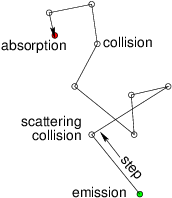
A particle executes a random walk<a 
id="random_walk121663"></a> through the
matter, illustrated in Fig.&nbsp;<a href="chap12.xml#randomwalkl">12.1</a>. It travels a certain
distance in a straight line, then collides. After the collision it has
a different direction and speed. It takes another step in the new
direction, generally with a different distance, to the next
collision. Eventually the particle has an absorbing collision, or
leaves the system, or becomes so degraded (for example in energy) that
it need no-longer be tracked. The walk ends.

<div class="p"><!----></div>
     <a id="tth_sEc12.1.1"></a><h3>
12.1.1&nbsp;&nbsp;Random walk step length</h3>

<div class="p"><!----></div>
The length of any of the steps between collisions is random. For any
collision process, the average number of collisions a particle has per
unit length corresponding to that process, which we'll label <math xmlns="http://www.w3.org/1998/Math/MathML">
<mrow><mi>j</mi></mrow></math>, is <math xmlns="http://www.w3.org/1998/Math/MathML">
<mrow>
<msub><mrow><mi>n</mi></mrow><mrow><mi>j</mi></mrow>
</msub>

<msub><mrow><mi mathvariant="italic">&sigma;</mi></mrow><mrow><mi>j</mi></mrow>
</msub>
</mrow></math>, where <math xmlns="http://www.w3.org/1998/Math/MathML">
<mrow>
<msub><mrow><mi mathvariant="italic">&sigma;</mi></mrow><mrow><mi>j</mi></mrow>
</msub>
</mrow></math> is the cross-section, and <math xmlns="http://www.w3.org/1998/Math/MathML">
<mrow>
<msub><mrow><mi>n</mi></mrow><mrow><mi>j</mi></mrow>
</msub>
</mrow></math> is the
density in the matter of the target species that has collisions of
type <math xmlns="http://www.w3.org/1998/Math/MathML">
<mrow><mi>j</mi></mrow></math>. For example, if the particles are neutrons and the process
is uranium nuclear fission, <math xmlns="http://www.w3.org/1998/Math/MathML">
<mrow>
<msub><mrow><mi>n</mi></mrow><mrow><mi>j</mi></mrow>
</msub>
</mrow></math> would be the density of uranium
nuclei. The average total number of collisions of all types per unit
path length is therefore<a 
id="step_length121664"></a>
<a id="colperlen">
</a><br />
<table width="100%"><tr><td align="center">
    <math xmlns="http://www.w3.org/1998/Math/MathML">
    <mstyle displaystyle="true"><mrow>
<msub><mrow><mi mathvariant="italic">&Sigma;</mi></mrow><mrow><mi>t</mi></mrow>
</msub>
<mo>=</mo>
<munder><mo>&sum;</mo><mrow><mi>j</mi></mrow>
</munder>

<msub><mrow><mi>n</mi></mrow><mrow><mi>j</mi></mrow>
</msub>

<msub><mrow><mi mathvariant="italic">&sigma;</mi></mrow><mrow><mi>j</mi></mrow>
</msub>
<mo>,</mo></mrow>
    </mstyle></math></td><td width="1">
    <math xmlns="http://www.w3.org/1998/Math/MathML">
    <mstyle displaystyle="true"><mrow><mo stretchy="false">(</mo><mn>12</mn><mo>.</mo><mn>1</mn><mo stretchy="false">)</mo></mrow>
    </mstyle></math>
</td></tr></table>


where the sum is over all possible collision processes. Once again
<math xmlns="http://www.w3.org/1998/Math/MathML">
<mrow>
<msub><mrow><mi mathvariant="italic">&Sigma;</mi></mrow><mrow><mi>t</mi></mrow>
</msub>
</mrow></math><a 
id="macroscopic_cross-section121665"></a> is an inverse
attenuation-length<a 
id="attenuation-length121666"></a>.

<div class="p"><!----></div>
How far does a particle go before having a collision?  Well, even for
particles with identical position and velocity, it varies
statistically in an unpredictable way. However, the probability of
having a collision in the small distance <math xmlns="http://www.w3.org/1998/Math/MathML">
<mrow><mi fontstyle="italic">l</mi><mo>&rarr;</mo><mi fontstyle="italic">l</mi><mo>+</mo><mi>d</mi><mi fontstyle="italic">l</mi></mrow></math>, given that the
particle started at <math xmlns="http://www.w3.org/1998/Math/MathML">
<mrow><mi fontstyle="italic">l</mi></mrow></math> (in other words, earlier collisions are
excluded), is <math xmlns="http://www.w3.org/1998/Math/MathML">
<mrow>
<msub><mrow><mi mathvariant="italic">&Sigma;</mi></mrow><mrow><mi>t</mi></mrow>
</msub>
<mi mathvariant="italic">dl</mi></mrow></math>. This incremental collision probability
<math xmlns="http://www.w3.org/1998/Math/MathML">
<mrow>
<msub><mrow><mi mathvariant="italic">&Sigma;</mi></mrow><mrow><mi>t</mi></mrow>
</msub>
<mi>d</mi><mi fontstyle="italic">l</mi></mrow></math> is independent of prior events.

<div class="p"><!----></div>
<a id="tth_fIg12.2">
</a>   <img src="figures/survivalprob.png" alt="figures/survivalprob.png" /><a id="survivalprob">
</a>
  
<div style="text-align:center">Figure 12.2: The probability, <math xmlns="http://www.w3.org/1998/Math/MathML">
<mrow>
<mover><mrow><mi>P</mi></mrow>
<mo>&OverBar;</mo></mover>
<mo stretchy="false">(</mo><mi>l</mi><mo stretchy="false">)</mo></mrow></math>, of survival without a
    collision to position <math xmlns="http://www.w3.org/1998/Math/MathML">
<mrow><mi>l</mi></mrow></math> decreases by a multiplicative factor
    <math xmlns="http://www.w3.org/1998/Math/MathML">
<mrow><mn>1</mn><mo>-</mo>
<msub><mrow><mi mathvariant="italic">&Sigma;</mi></mrow><mrow><mi>t</mi></mrow>
</msub>
<mi mathvariant="italic">dl</mi></mrow></math> in an increment <math xmlns="http://www.w3.org/1998/Math/MathML">
<mrow><mi mathvariant="italic">dl</mi></mrow></math>. <a id="survivalprobl">
</a></div>

<div class="p"><!----></div>
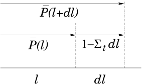
 Therefore (refer to Fig.&nbsp;<a href="chap12.xml#survivalprobl">12.2</a>) if the
probability that the particle survives at least as far as <math xmlns="http://www.w3.org/1998/Math/MathML">
<mrow><mi fontstyle="italic">l</mi></mrow></math> <em>without</em>
a collision is <math xmlns="http://www.w3.org/1998/Math/MathML">
<mrow>
<mover><mrow><mi>P</mi></mrow>
<mo>&OverBar;</mo></mover>
<mo stretchy="false">(</mo><mi fontstyle="italic">l</mi><mo stretchy="false">)</mo></mrow></math>, then the probability that it survives at
least as far as <math xmlns="http://www.w3.org/1998/Math/MathML">
<mrow><mi fontstyle="italic">l</mi><mo>+</mo><mi>d</mi><mi fontstyle="italic">l</mi></mrow></math> is the product of <math xmlns="http://www.w3.org/1998/Math/MathML">
<mrow>
<mover><mrow><mi>P</mi></mrow>
<mo>&OverBar;</mo></mover>
<mo stretchy="false">(</mo><mi fontstyle="italic">l</mi><mo stretchy="false">)</mo></mrow></math> times the
probability <math xmlns="http://www.w3.org/1998/Math/MathML">
<mrow><mn>1</mn><mo>-</mo>
<msub><mrow><mi mathvariant="italic">&Sigma;</mi></mrow><mrow><mi>t</mi></mrow>
</msub>
<mi>d</mi><mi fontstyle="italic">l</mi></mrow></math> that it <em>does not</em> have a collision in
<math xmlns="http://www.w3.org/1998/Math/MathML">
<mrow><mi>d</mi><mi fontstyle="italic">l</mi></mrow></math>:
<a id="probdiff">
</a><br />
<table width="100%"><tr><td align="center">
    <math xmlns="http://www.w3.org/1998/Math/MathML">
    <mstyle displaystyle="true"><mrow>
<mover><mrow><mi>P</mi></mrow>
<mo>&OverBar;</mo></mover>
<mo stretchy="false">(</mo><mi fontstyle="italic">l</mi><mo>+</mo><mi>d</mi><mi fontstyle="italic">l</mi><mo stretchy="false">)</mo><mo>=</mo>
<mover><mrow><mi>P</mi></mrow>
<mo>&OverBar;</mo></mover>
<mo stretchy="false">(</mo><mi fontstyle="italic">l</mi><mo stretchy="false">)</mo><mo stretchy="false">(</mo><mn>1</mn><mo>-</mo>
<msub><mrow><mi mathvariant="italic">&Sigma;</mi></mrow><mrow><mi>t</mi></mrow>
</msub>
<mi>d</mi><mi fontstyle="italic">l</mi><mo stretchy="false">)</mo></mrow>
    </mstyle></math></td><td width="1">
    <math xmlns="http://www.w3.org/1998/Math/MathML">
    <mstyle displaystyle="true"><mrow><mo stretchy="false">(</mo><mn>12</mn><mo>.</mo><mn>2</mn><mo stretchy="false">)</mo></mrow>
    </mstyle></math>
</td></tr></table>


Hence
<a id="diffprob">
</a><br />
<table width="100%"><tr><td align="center">
    <math xmlns="http://www.w3.org/1998/Math/MathML">
    <mstyle displaystyle="true"><mrow>
<mfrac><mrow>
<mover><mrow><mi>P</mi></mrow>
<mo>&OverBar;</mo></mover>
<mo stretchy="false">(</mo><mi fontstyle="italic">l</mi><mo>+</mo><mi>d</mi><mi fontstyle="italic">l</mi><mo stretchy="false">)</mo><mo>-</mo>
<mover><mrow><mi>P</mi></mrow>
<mo>&OverBar;</mo></mover>
<mo stretchy="false">(</mo><mi fontstyle="italic">l</mi><mo stretchy="false">)</mo></mrow>
<mrow><mi>d</mi><mi fontstyle="italic">l</mi></mrow>
</mfrac>
<mi>&emsp;</mi>
<munder><mrow><mo>&rarr;</mo></mrow>
<mrow><mi mathvariant="italic">dl</mi><mo>&rarr;</mo><mn>0</mn></mrow>
</munder>
<mi>&ensp;</mi>
<mfrac><mrow><mi>d</mi>
<mover><mrow><mi>P</mi></mrow>
<mo>&OverBar;</mo></mover>
</mrow>
<mrow><mi>d</mi><mi fontstyle="italic">l</mi></mrow>
</mfrac>
<mo>=</mo><mo>-</mo>
<msub><mrow><mi mathvariant="italic">&Sigma;</mi></mrow><mrow><mi>t</mi></mrow>
</msub>

<mover><mrow><mi>P</mi></mrow>
<mo>&OverBar;</mo></mover>
<mo>.</mo></mrow>
    </mstyle></math></td><td width="1">
    <math xmlns="http://www.w3.org/1998/Math/MathML">
    <mstyle displaystyle="true"><mrow><mo stretchy="false">(</mo><mn>12</mn><mo>.</mo><mn>3</mn><mo stretchy="false">)</mo></mrow>
    </mstyle></math>
</td></tr></table>


The solution of this differential equation is 
<a id="Pexpsigma">
</a><br />
<table width="100%"><tr><td align="center">
    <math xmlns="http://www.w3.org/1998/Math/MathML">
    <mstyle displaystyle="true"><mrow>
<mover><mrow><mi>P</mi></mrow>
<mo>&OverBar;</mo></mover>
<mo stretchy="false">(</mo><mi fontstyle="italic">l</mi><mo stretchy="false">)</mo><mo>=</mo><mi>exp</mi><mo stretchy="false">(</mo><mo>-</mo>
<msubsup><mrow><mo>&int;</mo></mrow><mrow><mn>0</mn> </mrow>
<mrow><mi>l</mi></mrow></msubsup>

<msub><mrow><mi mathvariant="italic">&Sigma;</mi></mrow><mrow><mi>t</mi></mrow>
</msub>
<mi>d</mi><mi fontstyle="italic">l</mi><mo stretchy="false">)</mo><mo>,</mo></mrow>
    </mstyle></math></td><td width="1">
    <math xmlns="http://www.w3.org/1998/Math/MathML">
    <mstyle displaystyle="true"><mrow><mo stretchy="false">(</mo><mn>12</mn><mo>.</mo><mn>4</mn><mo stretchy="false">)</mo></mrow>
    </mstyle></math>
</td></tr></table>


where <math xmlns="http://www.w3.org/1998/Math/MathML">
<mrow><mi fontstyle="italic">l</mi></mrow></math> is measured from the starting position, so <math xmlns="http://www.w3.org/1998/Math/MathML">
<mrow>
<mover><mrow><mi>P</mi></mrow>
<mo>&OverBar;</mo></mover>
<mo stretchy="false">(</mo><mn>0</mn><mo stretchy="false">)</mo><mo>=</mo><mn>1</mn></mrow></math>. Another equivalent way to define <math xmlns="http://www.w3.org/1998/Math/MathML">
<mrow>
<mover><mrow><mi>P</mi></mrow>
<mo>&OverBar;</mo></mover>
<mo stretchy="false">(</mo><mi fontstyle="italic">l</mi><mo stretchy="false">)</mo></mrow></math> is: the
probability that the first collision is <em>not</em> in the interval
<math xmlns="http://www.w3.org/1998/Math/MathML">
<mrow><mn>0</mn><mo>&rarr;</mo><mi fontstyle="italic">l</mi></mrow></math>.  The complement <math xmlns="http://www.w3.org/1998/Math/MathML">
<mrow><mi>P</mi><mo stretchy="false">(</mo><mi fontstyle="italic">l</mi><mo stretchy="false">)</mo><mo>=</mo><mn>1</mn><mo>-</mo>
<mover><mrow><mi>P</mi></mrow>
<mo>&OverBar;</mo></mover>
<mo stretchy="false">(</mo><mi fontstyle="italic">l</mi><mo stretchy="false">)</mo></mrow></math> is therefore the
probability that the first collision <em>is</em> in <math xmlns="http://www.w3.org/1998/Math/MathML">
<mrow><mn>0</mn><mo>&rarr;</mo><mi fontstyle="italic">l</mi></mrow></math>. In other
words, <math xmlns="http://www.w3.org/1998/Math/MathML">
<mrow><mi>P</mi><mo stretchy="false">(</mo><mi fontstyle="italic">l</mi><mo stretchy="false">)</mo><mo>=</mo><mn>1</mn><mo>-</mo>
<mover><mrow><mi>P</mi></mrow>
<mo>&OverBar;</mo></mover>
<mo stretchy="false">(</mo><mi fontstyle="italic">l</mi><mo stretchy="false">)</mo></mrow></math> is a cumulative probability. It is the
integral of the probability distribution <math xmlns="http://www.w3.org/1998/Math/MathML">
<mrow><mi>p</mi><mo stretchy="false">(</mo><mi fontstyle="italic">l</mi><mo stretchy="false">)</mo><mi>d</mi><mi fontstyle="italic">l</mi></mrow></math> that the (first)
collision takes place in <math xmlns="http://www.w3.org/1998/Math/MathML">
<mrow><mi>d</mi><mi fontstyle="italic">l</mi></mrow></math> at <math xmlns="http://www.w3.org/1998/Math/MathML">
<mrow><mi fontstyle="italic">l</mi></mrow></math>; so:
<a id="colpdist">
</a><br />
<table width="100%"><tr><td align="center">
    <math xmlns="http://www.w3.org/1998/Math/MathML">
    <mstyle displaystyle="true"><mrow><mi>p</mi><mo stretchy="false">(</mo><mi fontstyle="italic">l</mi><mo stretchy="false">)</mo><mo>=</mo>
<mfrac><mrow><mi mathvariant="italic">dP</mi></mrow>
<mrow><mi>d</mi><mi fontstyle="italic">l</mi></mrow>
</mfrac>
<mo>=</mo><mo>-</mo>
<mfrac><mrow><mi>d</mi>
<mover><mrow><mi>P</mi></mrow>
<mo>&OverBar;</mo></mover>
</mrow>
<mrow><mi>d</mi><mi fontstyle="italic">l</mi></mrow>
</mfrac>
<mo>=</mo>
<msub><mrow><mi mathvariant="italic">&Sigma;</mi></mrow><mrow><mi>t</mi></mrow>
</msub>

<mover><mrow><mi>P</mi></mrow>
<mo>&OverBar;</mo></mover>
<mo>=</mo>
<msub><mrow><mi mathvariant="italic">&Sigma;</mi></mrow><mrow><mi>t</mi></mrow>
</msub>
<mi>exp</mi><mo stretchy="false">(</mo><mo>-</mo>
<msubsup><mrow><mo>&int;</mo></mrow><mrow><mn>0</mn> </mrow>
<mrow><mi>l</mi></mrow></msubsup>

<msub><mrow><mi mathvariant="italic">&Sigma;</mi></mrow><mrow><mi>t</mi></mrow>
</msub>
<mi>d</mi><mi fontstyle="italic">l</mi><mo stretchy="false">)</mo><mo>.</mo></mrow>
    </mstyle></math></td><td width="1">
    <math xmlns="http://www.w3.org/1998/Math/MathML">
    <mstyle displaystyle="true"><mrow><mo stretchy="false">(</mo><mn>12</mn><mo>.</mo><mn>5</mn><mo stretchy="false">)</mo></mrow>
    </mstyle></math>
</td></tr></table>


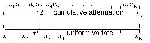
To decide statistically where the first
collision<a 
id="collision_first121667"></a> takes place for any specific
particle, therefore, we simply draw a random number (uniform variate)
and select <math xmlns="http://www.w3.org/1998/Math/MathML">
<mrow><mi fontstyle="italic">l</mi></mrow></math> from the cumulative distribution <math xmlns="http://www.w3.org/1998/Math/MathML">
<mrow><mi>P</mi><mo stretchy="false">(</mo><mi fontstyle="italic">l</mi><mo stretchy="false">)</mo></mrow></math> as
explained in section <a href="chap11.xml#comprandsel">11.2</a> and illustrated in Fig.&nbsp;<a href="chap11.xml#Pselect">11.1</a>.  If we are dealing with a step in which <math xmlns="http://www.w3.org/1998/Math/MathML">
<mrow>
<msub><mrow><mi mathvariant="italic">&Sigma;</mi></mrow><mrow><mi>t</mi></mrow>
</msub>
</mrow></math> can
be taken as uniform, then <math xmlns="http://www.w3.org/1998/Math/MathML">
<mrow><mi>P</mi><mo stretchy="false">(</mo><mi fontstyle="italic">l</mi><mo stretchy="false">)</mo><mo>=</mo><mn>1</mn><mo>-</mo><mi>exp</mi><mo stretchy="false">(</mo><mo>-</mo>
<msub><mrow><mi mathvariant="italic">&Sigma;</mi></mrow><mrow><mi>t</mi></mrow>
</msub>
<mi fontstyle="italic">l</mi><mo stretchy="false">)</mo></mrow></math>, and the
cumulative function can be inverted analytically as
<math xmlns="http://www.w3.org/1998/Math/MathML">
<mrow><mi fontstyle="italic">l</mi><mo stretchy="false">(</mo><mi>P</mi><mo stretchy="false">)</mo><mo>=</mo><mo>-</mo><mi>ln</mi><mo stretchy="false">(</mo><mn>1</mn><mo>-</mo><mi>P</mi><mo stretchy="false">)</mo><mo stretchy="false">/</mo>
<msub><mrow><mi mathvariant="italic">&Sigma;</mi></mrow><mrow><mi>t</mi></mrow>
</msub>
</mrow></math>.

<div class="p"><!----></div>
     <a id="tth_sEc12.1.2"></a><h3>
12.1.2&nbsp;&nbsp;Collision type and parameters</h3>

<div class="p"><!----></div>
Having decided where the next collision happens, we need to decide
what sort of collision<a 
id="collision_type121668"></a> it is. The local rate at
which each type <math xmlns="http://www.w3.org/1998/Math/MathML">
<mrow><mi>j</mi></mrow></math> of collision is occuring is <math xmlns="http://www.w3.org/1998/Math/MathML">
<mrow>
<msub><mrow><mi>n</mi></mrow><mrow><mi>j</mi></mrow>
</msub>

<msub><mrow><mi mathvariant="italic">&sigma;</mi></mrow><mrow><mi>j</mi></mrow>
</msub>
</mrow></math> and the
sum of all <math xmlns="http://www.w3.org/1998/Math/MathML">
<mrow>
<msub><mrow><mi>n</mi></mrow><mrow><mi>j</mi></mrow>
</msub>

<msub><mrow><mi mathvariant="italic">&sigma;</mi></mrow><mrow><mi>j</mi></mrow>
</msub>
</mrow></math> is <math xmlns="http://www.w3.org/1998/Math/MathML">
<mrow>
<msub><mrow><mi mathvariant="italic">&Sigma;</mi></mrow><mrow><mi>t</mi></mrow>
</msub>
</mrow></math>. Therefore the fraction of
collisions that is of type <math xmlns="http://www.w3.org/1998/Math/MathML">
<mrow><mi>j</mi></mrow></math> is <math xmlns="http://www.w3.org/1998/Math/MathML">
<mrow>
<msub><mrow><mi>n</mi></mrow><mrow><mi>j</mi></mrow>
</msub>

<msub><mrow><mi mathvariant="italic">&sigma;</mi></mrow><mrow><mi>j</mi></mrow>
</msub>
<mo stretchy="false">/</mo>
<msub><mrow><mi mathvariant="italic">&Sigma;</mi></mrow><mrow><mi>t</mi></mrow>
</msub>
</mrow></math>.

<div class="p"><!----></div>
<a id="tth_fIg12.3">
</a>   <img src="figures/typelist.png" alt="figures/typelist.png" /><a id="typelist">
</a>
  
<div style="text-align:center">Figure 12.3: Deciding the collision type based upon a random number <math xmlns="http://www.w3.org/1998/Math/MathML">
<mrow><mi>x</mi></mrow></math>.<a id="typelistl">
</a></div>

<div class="p"><!----></div>
If we regard all the
possible types of collisions as arrayed in a long list, illustrated in
Fig.&nbsp;<a href="chap12.xml#typelistl">12.3</a>, and to each
type is assigned a real number <math xmlns="http://www.w3.org/1998/Math/MathML">
<mrow>
<msub><mrow><mi>x</mi></mrow><mrow><mi>j</mi></mrow>
</msub>
</mrow></math> such that
<math xmlns="http://www.w3.org/1998/Math/MathML">
<mrow>
<msub><mrow><mi>x</mi></mrow><mrow><mi>j</mi><mo>+</mo><mn>1</mn></mrow>
</msub>
<mo>=</mo>
<msub><mrow><mi>x</mi></mrow><mrow><mi>j</mi></mrow>
</msub>
<mo>+</mo>
<msub><mrow><mi>n</mi></mrow><mrow><mi>j</mi></mrow>
</msub>

<msub><mrow><mi mathvariant="italic">&sigma;</mi></mrow><mrow><mi>j</mi></mrow>
</msub>
<mo stretchy="false">/</mo>
<msub><mrow><mi mathvariant="italic">&Sigma;</mi></mrow><mrow><mi>t</mi></mrow>
</msub>
</mrow></math>, i.e.
<a id="xpsum">
</a><br />
<table width="100%"><tr><td align="center">
    <math xmlns="http://www.w3.org/1998/Math/MathML">
    <mstyle displaystyle="true"><mrow>
<msub><mrow><mi>x</mi></mrow><mrow><mi>j</mi></mrow>
</msub>
<mo>=</mo>
<munderover><mo>&sum;</mo><mrow><mi>i</mi><mo>=</mo><mn>1</mn> </mrow>
<mrow><mi>j</mi><mo>-</mo><mn>1</mn></mrow></munderover>
<msub><mrow><mi>n</mi></mrow><mrow><mi>i</mi></mrow>
</msub>

<msub><mrow><mi mathvariant="italic">&sigma;</mi></mrow><mrow><mi>i</mi></mrow>
</msub>
<mo stretchy="false">/</mo>
<msub><mrow><mi mathvariant="italic">&Sigma;</mi></mrow><mrow><mi>t</mi></mrow>
</msub>
<mo>,</mo></mrow>
    </mstyle></math></td><td width="1">
    <math xmlns="http://www.w3.org/1998/Math/MathML">
    <mstyle displaystyle="true"><mrow><mo stretchy="false">(</mo><mn>12</mn><mo>.</mo><mn>6</mn><mo stretchy="false">)</mo></mrow>
    </mstyle></math>
</td></tr></table>


then a single random draw <math xmlns="http://www.w3.org/1998/Math/MathML">
<mrow><mi>x</mi></mrow></math> determines <math xmlns="http://www.w3.org/1998/Math/MathML">
<mrow><mi>j</mi></mrow></math> by the condition <math xmlns="http://www.w3.org/1998/Math/MathML">
<mrow>
<msub><mrow><mi>x</mi></mrow><mrow><mi>j</mi></mrow>
</msub>
<mo>&le;</mo><mi>x</mi><mo>&lt;</mo>
<msub><mrow><mi>x</mi></mrow><mrow><mi>j</mi><mo>+</mo><mn>1</mn></mrow>
</msub>
</mrow></math>. This is just the process of drawing from a discrete
probability distribution. Our previous examples were the Poisson
distribution, and the weighting of discrete particles for flux injection.

<div class="p"><!----></div>
Once having decided upon the collision process <math xmlns="http://www.w3.org/1998/Math/MathML">
<mrow><mi>j</mi></mrow></math>, there are
(usually) other parameters of the collision to be decided. For
example, if the collision is a scattering event, what is the
scattering angle and the corresponding new scattered velocity
<math xmlns="http://www.w3.org/1998/Math/MathML">
<mrow><mi mathvariant="bold-italic">v</mi></mrow></math> which serves<a href="footnote.xml#tthFtNtAHI" id="tthFrefAHI"><math xmlns="http://www.w3.org/1998/Math/MathML">
<mrow>
<msup><mrow></mrow><mrow><mn>78</mn></mrow>
</msup>
</mrow></math></a> to determine the starting condition of the next
step?  These random parameters are also determined by statistical
choice from the appropriate probability distributions, for example the
normalized differential<a 
id="scattering_angle121669"></a> cross-section per unit scattering angle.

<div class="p"><!----></div>
     <a id="tth_sEc12.1.3"></a><h3>
12.1.3&nbsp;&nbsp;Iteration and New Particles</h3>

<div class="p"><!----></div>
Once the collision parameters have been decided, unless the event was an
absorption, the particle is restarted from the position of collision
with the new velocity and the next step is calculated. If the particle
is absorbed<a 
id="absorption121670"></a>, or escapes from the modelled region,
then instead we start a completely new particle. Where and how it is
started depends upon the sort of radiation transport problem we are
solving. If it is transport from a localized known source, then that
determines the initialization position, and its direction is
appropriately chosen.  If the matter is emitting, new particles can be
generated spread throughout the volume. Spontaneous
emission<a 
id="spontaneous_emission121671"></a>, arising independent of the level
of<a 
id="emission_spontaneous121672"></a> radiation in the medium, is simply a
distributed source. It serves to determine the distribution of brand
new particles, which are launched once all active particles have been
followed till absorbed or escaped. Examples of spontaneous emission
include radiation from excited atoms, spontaneous radioactive decays
giving gammas, or spontaneous fissions giving neutrons.  However,
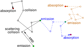
often the new particles are "stimulated"<a 
id="emission_stimulated121673"></a>
by collisions from the transporting particles. Fig.&nbsp;<a href="chap12.xml#lstimulated">12.4</a>
illustrates this process. The classic nuclear example is induced
fission producing additional neutrons. Stimulated emission arises as a
product of a certain type of collision.
<div class="p"><!----></div>
<a id="tth_fIg12.4">
</a> <img src="figures/generations.png" alt="figures/generations.png" /><a id="generations">
</a>
  
<div style="text-align:center">Figure 12.4: "Stimulated" emission is a source of new particles caused
    by the collisions of the old ones. It can multiply the particles
    through succeeding generations, as the new particles (different
    line styles) give rise themselves to additional
    emissions.<a id="lstimulated">
</a></div>

<div class="p"><!----></div>
Any additional particles produced by collisions must be tracked by the
same process as used for the original particle. They become new
tracks. In a serial code, the secondary particles must be initialized
and then set aside during the collision step. Then when the original
track ends by absorption or escape, the code must take up the job of
tracking the secondary particles. The secondary particles may generate
tertiary particles, which will also eventually be tracked. And so on.
Parallel code might offload the secondary and tertiary tracks to other
processors (or computational threads). 

<div class="p"><!----></div>
One might be concerned that we'll never get to the end if particles
are generated faster than they are lost. That's true; we won't. But
particle generation faster than loss corresponds to runaway physical
situation, for example a prompt supercritical reactor. So the
real-world will have problems much more troublesome than our
computational ones!

<div class="p"><!----></div>
 <a id="tth_sEc12.2"></a><h2>
12.2&nbsp;&nbsp;Tracking, Tallying and Statistical Uncertainty</h2>

<div class="p"><!----></div>
The purpose of a Monte Carlo simulation is generally to determine some
averaged bulk parameters of the radiation particles or the matter
itself. The sorts of parameters include, radiation flux as a function
of position, spectrum of particle energies, rate of occurrence of
certain types of collision, or resulting state of the matter through
which the radiation passes. To determine these sorts of quantities
requires keeping track of the passage of particles through the
relevant regions of space, and of the collisions that occur there.
The computational task of keeping track of events and contributions to
statistical quantities is often called "tallying"<a 
id="tally122674"></a>. 

<div class="p"><!----></div>
What is generally done is to divide the region of interest into a
managable number of discrete volumes, in which the tallies of interest
are going to be accumulated. Each time an event occurs in one of these
volumes, it is added to the tally. Then, provided a reasonably large
number of such events has occurred, the average rate of the occurrence
of events of interest can be obtained. For example, if we wish to know
the fission power distribution in a nuclear reactor, we would tally
the number of fission collisions occurring in each volume. Fission
reactions release on average a known amount of total energy <math xmlns="http://www.w3.org/1998/Math/MathML">
<mrow><mrow><mstyle fontfamily="helvetica">
<mi fontstyle="italic">E</mi></mstyle></mrow>
</mrow></math>. So if the number occuring in a particular volume <math xmlns="http://www.w3.org/1998/Math/MathML">
<mrow><mi>V</mi></mrow></math>, during a
time <math xmlns="http://www.w3.org/1998/Math/MathML">
<mrow><mi>T</mi></mrow></math> is <math xmlns="http://www.w3.org/1998/Math/MathML">
<mrow><mi>N</mi></mrow></math>, the fission power density is <math xmlns="http://www.w3.org/1998/Math/MathML">
<mrow><mi>N</mi><mrow><mstyle fontfamily="helvetica"><mi fontstyle="italic">E</mi></mstyle></mrow>
<mo stretchy="false">/</mo><mi mathvariant="italic">VT</mi></mrow></math>. 

<div class="p"><!----></div>
The number of computational random walks that we can afford to track
is usually far less than the number of events that would actually
happen in the physical system being modelled. Each computational
particle can be considered to represent a large number of actual
particles all doing the same thing. The much smaller computational
number leads to important statistical fluctuations, uncertainty, or
noise, that is a purely computational limitation.

<div class="p"><!----></div>

<b>The statistical uncertainty&nbsp;&nbsp;</b><a 
id="uncertainty_statistical122675"></a>
of a Monte Carlo<a 
id="statistical_uncertainty122676"></a> calculation is
generally determined by the observation that a sample of <math xmlns="http://www.w3.org/1998/Math/MathML">
<mrow><mi>N</mi></mrow></math> random
choices from a distribution (population) of standard deviation <math xmlns="http://www.w3.org/1998/Math/MathML">
<mrow><mi>S</mi></mrow></math> has
a sample mean <math xmlns="http://www.w3.org/1998/Math/MathML">
<mrow>
<msub><mrow><mi mathvariant="italic">&mu;</mi></mrow><mrow><mi>N</mi></mrow>
</msub>
</mrow></math> whose standard deviation is equal to the
standard error <math xmlns="http://www.w3.org/1998/Math/MathML">
<mrow><mi>S</mi><mo stretchy="false">/</mo><msqrt><mrow><mi>N</mi></mrow></msqrt></mrow></math>. Each tally event acts like single random
choice. Therefore for <math xmlns="http://www.w3.org/1998/Math/MathML">
<mrow><mi>N</mi></mrow></math> tally events the uncertainty in the quantity
to be determined is smaller than its intrinsic uncertainty or
statistical range by a factor <math xmlns="http://www.w3.org/1998/Math/MathML">
<mrow><mn>1</mn><mo stretchy="false">/</mo><msqrt><mrow><mi>N</mi></mrow></msqrt></mrow></math>. Put differently, suppose the
average rate of a certain type of statistically determined event is
constant, giving on average <math xmlns="http://www.w3.org/1998/Math/MathML">
<mrow><mi>N</mi></mrow></math> events in time <math xmlns="http://www.w3.org/1998/Math/MathML">
<mrow><mi>T</mi></mrow></math> then the number <math xmlns="http://www.w3.org/1998/Math/MathML">
<mrow><mi>n</mi></mrow></math>
of events in any particular time interval of length <math xmlns="http://www.w3.org/1998/Math/MathML">
<mrow><mi>T</mi></mrow></math> is governed by
a Poisson probability, eq.&nbsp;(<a href="chap11.xml#PoissonDist">11.15</a>) <math xmlns="http://www.w3.org/1998/Math/MathML">
<mrow><mi>p</mi><mo stretchy="false">(</mo><mi>n</mi><mo stretchy="false">)</mo><mo>=</mo><mi>exp</mi><mo stretchy="false">(</mo><mo>-</mo><mi>N</mi><mo stretchy="false">)</mo>
<msup><mrow><mi>N</mi></mrow><mrow><mi>n</mi></mrow>
</msup>
<mo stretchy="false">/</mo><mi>n</mi><mo>!</mo></mrow></math>. The standard deviation of this Poisson distribution
is <math xmlns="http://www.w3.org/1998/Math/MathML">
<mrow><msqrt><mrow><mi>N</mi></mrow></msqrt></mrow></math>. Therefore we obtain a precise estimate of the average rate of
events, <math xmlns="http://www.w3.org/1998/Math/MathML">
<mrow><mi>N</mi></mrow></math>, by using the number actually observed in a particular
case, <math xmlns="http://www.w3.org/1998/Math/MathML">
<mrow><mi>n</mi></mrow></math>, only if <math xmlns="http://www.w3.org/1998/Math/MathML">
<mrow><mi>N</mi></mrow></math> (and therefore <math xmlns="http://www.w3.org/1998/Math/MathML">
<mrow><mi>n</mi></mrow></math>) is a large number.

<div class="p"><!----></div>
The first conclusion is that we must not choose our discrete tallying
volumes too small. The smaller they are, the fewer events will occur
in them, and, therefore, the less statistically accurate will be the
estimate of the event rate.

<div class="p"><!----></div>
When tallying collisions<a 
id="collision_tally122677"></a>, the first thought one
might have is simply to put a check mark against each type of
collision for each volume element, whenever that exact type of event
occurs in it. The difficulty with this approach is that it will give
very poor statistics, because there are going to be too few check
marks. To get, say, 1% statistical uncertainty, we would need <math xmlns="http://www.w3.org/1998/Math/MathML">
<mrow>
<msup><mrow><mn>10</mn></mrow><mrow><mn>4</mn></mrow>
</msup>
</mrow></math>
check marks for each discrete volume. If the events are spread over,
say <math xmlns="http://www.w3.org/1998/Math/MathML">
<mrow>
<msup><mrow><mn>100</mn></mrow><mrow><mn>3</mn></mrow>
</msup>
</mrow></math> volumes, we would need <math xmlns="http://www.w3.org/1998/Math/MathML">
<mrow>
<msup><mrow><mn>10</mn></mrow><mrow><mn>10</mn></mrow>
</msup>
</mrow></math> total collisions <em>of
  each relevant type</em>. For, say, 100 collision types we are already up
to <math xmlns="http://www.w3.org/1998/Math/MathML">
<mrow>
<msup><mrow><mn>10</mn></mrow><mrow><mn>12</mn></mrow>
</msup>
</mrow></math> collisions. The cost is very great. But we can do better
than this na&#239;ve check-box approach.

<div class="p"><!----></div>
One thing we can do with negligible extra effort is to add to the
tally for <em>every</em> type of collision, whenever <em>any</em>
collision happens. To make this work, we must add a variable amount to
the tally, not just 1 (not just a check mark). The amount we should
add to each collision-type tally, is just the fraction of all
collisions that is of that type, namely <math xmlns="http://www.w3.org/1998/Math/MathML">
<mrow>
<msub><mrow><mi>n</mi></mrow><mrow><mi>j</mi></mrow>
</msub>

<msub><mrow><mi mathvariant="italic">&sigma;</mi></mrow><mrow><mi>j</mi></mrow>
</msub>
<mo stretchy="false">/</mo>
<msub><mrow><mi mathvariant="italic">&Sigma;</mi></mrow><mrow><mi>t</mi></mrow>
</msub>
</mrow></math>. Of
course these fractional values should be evaluated with values of
<math xmlns="http://www.w3.org/1998/Math/MathML">
<mrow>
<msub><mrow><mi>n</mi></mrow><mrow><mi>j</mi></mrow>
</msub>
</mrow></math> corresponding to the local volume, and at the velocity of the
particle being considered (which affects <math xmlns="http://www.w3.org/1998/Math/MathML">
<mrow>
<msub><mrow><mi mathvariant="italic">&sigma;</mi></mrow><mrow><mi>j</mi></mrow>
</msub>
</mrow></math>). This process
will produce, on average, the same correct collision
tally value, but will do so with a total number of contributions bigger by
a factor equal to the number of collision types. That substantially improves the
statistics.
<div class="p"><!----></div>
<a id="tth_fIg12.5">
</a>   <img src="figures/volumedisc.png" alt="figures/volumedisc.png" /><a id="volumedisc">
</a>
  
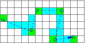
<div style="text-align:center">Figure 12.5: Tallying is done in discrete volumes. One can tally every
    collision(green) but if the steps are larger than the
    volumes, it gives better statistics to tally every volume the
    particle passes through(blue).<a id="volumediscl">
</a></div>

<div class="p"><!----></div>
A further statistical advantage is obtained by tallying more than just
collisions. If we want particle flux properties, as well as the
effects on the matter, we need to tally not just collisions, but also
the average flux density in all the discrete volumes. That requires us
to determine for every volume, every passage <math xmlns="http://www.w3.org/1998/Math/MathML">
<mrow><mi>i</mi></mrow></math> of a particle through
it, the fractional time <math xmlns="http://www.w3.org/1998/Math/MathML">
<mrow><mi mathvariant="italic">&Delta;</mi>
<msub><mrow><mi>t</mi></mrow><mrow><mi>i</mi></mrow>
</msub>
</mrow></math> that it spends in the volume, and
the speed <math xmlns="http://www.w3.org/1998/Math/MathML">
<mrow>
<msub><mrow><mi>v</mi></mrow><mrow><mi>i</mi></mrow>
</msub>
</mrow></math> at which it passed through. See Fig.&nbsp;<a href="chap12.xml#volumediscl">12.5</a>. When the simulation has been tracked for a
sufficient number of particles, the density of particles in the volume
is proportional to the sum <math xmlns="http://www.w3.org/1998/Math/MathML">
<mrow>
<munder><mo>&sum;</mo><mrow><mi>i</mi></mrow>
</munder>
<mi mathvariant="italic">&Delta;</mi>
<msub><mrow><mi>t</mi></mrow><mrow><mi>i</mi></mrow>
</msub>
</mrow></math> and the scalar flux
density<a href="footnote.xml#tthFtNtAHJ" id="tthFrefAHJ"><math xmlns="http://www.w3.org/1998/Math/MathML">
<mrow>
<msup><mrow></mrow><mrow><mn>79</mn></mrow>
</msup>
</mrow></math></a> to <math xmlns="http://www.w3.org/1998/Math/MathML">
<mrow>
<munder><mo>&sum;</mo><mrow><mi>i</mi></mrow>
</munder>

<msub><mrow><mi>v</mi></mrow><mrow><mi>i</mi></mrow>
</msub>
<mi mathvariant="italic">&Delta;</mi>
<msub><mrow><mi>t</mi></mrow><mrow><mi>i</mi></mrow>
</msub>
</mrow></math>. If collisional lengths (the length of the random walk step) are
substantially larger than the size of the discrete volumes, then there
are more contributions to the flux property tallies than there are
walk steps, i.e.&nbsp;modelled collisions. The statistical accuracy of the
flux density measurement is then better than the collision tallies
(even when all collision types are tallied for every collision) by a
factor approximately equal to the ratio of collision step length to
discrete volume side-length. Therefore it may be worth the effort to
keep a tally of the total contribution to collisions of type <math xmlns="http://www.w3.org/1998/Math/MathML">
<mrow><mi>j</mi></mrow></math> that
we care about from every track that passes through every volume. In
other words, for each volume, to obtain the sum over all passages <math xmlns="http://www.w3.org/1998/Math/MathML">
<mrow><mi>i</mi></mrow></math>:
<math xmlns="http://www.w3.org/1998/Math/MathML">
<mrow>
<munder><mo>&sum;</mo><mrow><mi>i</mi></mrow>
</munder>
<mi mathvariant="italic">&Delta;</mi>
<msub><mrow><mi>t</mi></mrow><mrow><mi>i</mi></mrow>
</msub>

<msub><mrow><mi>v</mi></mrow><mrow><mi>i</mi></mrow>
</msub>

<msub><mrow><mi>n</mi></mrow><mrow><mi>j</mi></mrow>
</msub>

<msub><mrow><mi mathvariant="italic">&sigma;</mi></mrow><mrow><mi>j</mi></mrow>
</msub>
</mrow></math>. The extra cost of this process
is the geometric task of determining the length of a line during which
it is inside a particular volume. But if that task is necessary
anyway, because flux properties are desired, then it is no more work
to tally the collisional probabilities in this way.

<div class="p"><!----></div>

<b>Importance weighting&nbsp;&nbsp;</b><a 
id="weighting_importance122678"></a>
Another<a 
id="importance_weighting122679"></a> aspect of statistical accuracy
relates to the choice of initial distribution of particles, especially
in velocity space. In some transport problems, it might be that the
particles that penetrate a large distance away from their source are
predominantly the high energy particles, perhaps those quite far out
on the tail of a birth velocity distribution that has the bulk of its
particles at low energy. The most straightforward way to represent the
transport problem is to launch particles in proportion to their
physical birth distribution. Each computational particle then
represents the same number of physical particles. But this choice
might mean there are very few of the high-energy particles that
determine the flux far from the source. If so, then the statistical
uncertainty of the far flux is going to be great.
<div class="p"><!----></div>
<a id="tth_fIg12.6">
</a>   <img src="figures/importance.png" alt="figures/importance.png" /><a id="importance">
</a>
  
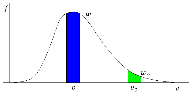
<div style="text-align:center">Figure 12.6: If all particles have the same weight, there are many more
    representing bulk velocities (<math xmlns="http://www.w3.org/1998/Math/MathML">
<mrow>
<msub><mrow><mi>v</mi></mrow><mrow><mn>1</mn></mrow>
</msub>
</mrow></math>) than tail velocities
    (<math xmlns="http://www.w3.org/1998/Math/MathML">
<mrow>
<msub><mrow><mi>v</mi></mrow><mrow><mn>2</mn></mrow>
</msub>
</mrow></math>). Improved statistical representation of the tail is
    obtained by giving the tail velocities lower weight <math xmlns="http://www.w3.org/1998/Math/MathML">
<mrow>
<msub><mrow><mi>w</mi></mrow><mrow><mn>2</mn></mrow>
</msub>
</mrow></math>. If the
    weights are proportional to <math xmlns="http://www.w3.org/1998/Math/MathML">
<mrow><mi>f</mi></mrow></math> then equal numbers of particles
    are assigned to equal velocity ranges.<a id="importancel">
</a></div>

<div class="p"><!----></div>
It is possible to compensate for this problem by <em>weighting</em> the
particles, illustrated by Fig.&nbsp;<a href="chap12.xml#importancel">12.6</a>. One can obtain
better far-flux statistics by launching more of the high energy
particles than would be implied by their probability distribution, but
compensating for the statistical excess by an importance weighting <math xmlns="http://www.w3.org/1998/Math/MathML">
<mrow><mi>w</mi></mrow></math>
that is inversely proportional to the factor by which the particle
number has exceeded the probability distribution. For a weighted
particle's subsequent random walk, and for any additional particles
emitted in response to collisions of the particle, the contribution
made to any flux or reaction rate is then multiplied by
<math xmlns="http://www.w3.org/1998/Math/MathML">
<mrow><mi>w</mi></mrow></math>. Consequently the total flux calculated anywhere has the correct
average contribution from all types of initial particles.  But there
are more actual contributions (of lower weight) from
high-initial-energy particles than there otherwise would be. This has
the effect of reducing the statistical uncertainty of flux that happens
to depend upon high energy birth particles by transferring some of the
computational effort to them from lower energy birth particles.

<div class="p"><!----></div>
Importance weighting is immediately accommodated during the tallying
process by adding contributions to the various flux tallies that are
the same as have been previously given - except: each contribution
is multiplied by the weight <math xmlns="http://www.w3.org/1998/Math/MathML">
<mrow>
<msub><mrow><mi>w</mi></mrow><mrow><mi>i</mi></mrow>
</msub>
</mrow></math> of that particular particle. Thus
density becomes <math xmlns="http://www.w3.org/1998/Math/MathML">
<mrow><mo>&prop;</mo>
<msub><mrow><mi mathvariant="italic">&Sigma;</mi></mrow><mrow><mi>i</mi></mrow>
</msub>

<msub><mrow><mi>w</mi></mrow><mrow><mi>i</mi></mrow>
</msub>
<mi mathvariant="italic">&Delta;</mi>
<msub><mrow><mi>t</mi></mrow><mrow><mi>i</mi></mrow>
</msub>
</mrow></math> and scalar flux
density <math xmlns="http://www.w3.org/1998/Math/MathML">
<mrow><mo>&prop;</mo>
<msub><mrow><mi mathvariant="italic">&Sigma;</mi></mrow><mrow><mi>i</mi></mrow>
</msub>

<msub><mrow><mi>w</mi></mrow><mrow><mi>i</mi></mrow>
</msub>

<msub><mrow><mi>v</mi></mrow><mrow><mi>i</mi></mrow>
</msub>
<mi mathvariant="italic">&Delta;</mi>
<msub><mrow><mi>t</mi></mrow><mrow><mi>i</mi></mrow>
</msub>
</mrow></math>, and so on.

<div class="p"><!----></div>
The weight of a particle that is launched as a result of stimulated
emission is inherited from its parent. A newly launched particle of
the <math xmlns="http://www.w3.org/1998/Math/MathML">
<mrow><mi>n</mi></mrow></math>th generation inherently acquires the weight <math xmlns="http://www.w3.org/1998/Math/MathML">
<mrow>
<msub><mrow><mi>w</mi></mrow><mrow><mi>n</mi><mo>-</mo><mn>1</mn></mrow>
</msub>
</mrow></math> of the
particular previous generation particle whose collision caused the
launch. However, in the process of deciding the <math xmlns="http://www.w3.org/1998/Math/MathML">
<mrow><mi>n</mi></mrow></math>th generation's
initial velocity an extra launch weighting is accorded to it,
corresponding to its launch parameters; for example it might be
weighted proportional to the launch speed (or energy) probability
distribution <math xmlns="http://www.w3.org/1998/Math/MathML">
<mrow><mi>p</mi><mo stretchy="false">(</mo>
<msub><mrow><mi>v</mi></mrow><mrow><mi>n</mi></mrow>
</msub>
<mo stretchy="false">)</mo></mrow></math>. If so, then the weight of the newly launched
particle is
<a id="generationwt">
</a><br />
<table width="100%"><tr><td align="center">
    <math xmlns="http://www.w3.org/1998/Math/MathML">
    <mstyle displaystyle="true"><mrow>
<msub><mrow><mi>w</mi></mrow><mrow><mi>n</mi></mrow>
</msub>
<mo>=</mo>
<msub><mrow><mi>w</mi></mrow><mrow><mi>n</mi><mo>-</mo><mn>1</mn></mrow>
</msub>
<mi>p</mi><mo stretchy="false">(</mo>
<msub><mrow><mi>v</mi></mrow><mrow><mi>n</mi></mrow>
</msub>
<mo stretchy="false">)</mo><mo>.</mo></mrow>
    </mstyle></math></td><td width="1">
    <math xmlns="http://www.w3.org/1998/Math/MathML">
    <mstyle displaystyle="true"><mrow><mo stretchy="false">(</mo><mn>12</mn><mo>.</mo><mn>7</mn><mo stretchy="false">)</mo></mrow>
    </mstyle></math>
</td></tr></table>


This process of weight multiplication between generations causes a
<em>spreading of the weights</em>. The ratio of the maximum to minimum
weight of each succeeding generation is multiplied by the birth
weight-ratio; so the weight range ratio grows geometrically. When
there is a very large range between the minimum and the maximum
weight, it becomes a waste of time to track particles whose weight is
negligibly small. So after the simulation has run for some time
duration, special procedures must be applied to limit the range of
weights by removing particles of irrelevantly small weight.

<div class="p"><!----></div>
 <a id="tth_sEc12.3"></a><h2>
12.3&nbsp;&nbsp;Worked Example:  Density and Flux Tallies</h2>

<div class="p"><!----></div>
In a Monte Carlo calculation of radiation transport from a
source emitting at a fixed rate <math xmlns="http://www.w3.org/1998/Math/MathML">
<mrow><mi>R</mi></mrow></math> particles per second, tallies in
the surrounding region are kept for every transit of a cell by every
particle. The tally for density in a particular cell consists of
adding the time interval <math xmlns="http://www.w3.org/1998/Math/MathML">
<mrow><mi mathvariant="italic">&Delta;</mi>
<msub><mrow><mi>t</mi></mrow><mrow><mi>i</mi></mrow>
</msub>
</mrow></math> during which a particle is in
it, every time the cell is crossed.  The tally for flux density adds
up the time interval multiplied by speed: <math xmlns="http://www.w3.org/1998/Math/MathML">
<mrow>
<msub><mrow><mi>v</mi></mrow><mrow><mi>i</mi></mrow>
</msub>
<mi mathvariant="italic">&Delta;</mi>
<msub><mrow><mi>t</mi></mrow><mrow><mi>i</mi></mrow>
</msub>
</mrow></math>. After
launching and tracking to extinction a large number <math xmlns="http://www.w3.org/1998/Math/MathML">
<mrow><mi>N</mi></mrow></math> of random
emitted particles, the sums are
<br />
<table width="100%"><tr><td align="center">
    <math xmlns="http://www.w3.org/1998/Math/MathML">
    <mstyle displaystyle="true"><mrow>
<msub><mrow><mi>S</mi></mrow><mrow><mi>n</mi></mrow>
</msub>
<mo>=</mo>
<munder><mo>&sum;</mo><mrow><mi>i</mi></mrow>
</munder>
<mi mathvariant="italic">&Delta;</mi>
<msub><mrow><mi>t</mi></mrow><mrow><mi>i</mi></mrow>
</msub>
<mo>,</mo><mi>&emsp;&emsp;&emsp;&emsp;&emsp;&emsp;</mi>
<msub><mrow><mi>S</mi></mrow><mrow><mi mathvariant="italic">&phi;</mi></mrow>
</msub>
<mo>=</mo>
<munder><mo>&sum;</mo><mrow><mi>i</mi></mrow>
</munder>

<msub><mrow><mi>v</mi></mrow><mrow><mi>i</mi></mrow>
</msub>
<mi mathvariant="italic">&Delta;</mi>
<msub><mrow><mi>t</mi></mrow><mrow><mi>i</mi></mrow>
</msub>
<mo>.</mo></mrow>
    </mstyle></math>
</td></tr></table>
<br />

Deduce quantitative physical formulas for what the particle and flux
densities are (not just that they are proportional to these sums), and
the uncertainties in them, giving careful rationales.

<div class="p"><!----></div>
<br /> A total of <math xmlns="http://www.w3.org/1998/Math/MathML">
<mrow><mi>N</mi></mrow></math> particles tracked from the source (not
including the other particles arising from collisions that we also had
to track), is the number of particles that would be emitted in a
time <math xmlns="http://www.w3.org/1998/Math/MathML">
<mrow><mi>T</mi><mo>=</mo><mi>N</mi><mo stretchy="false">/</mo><mi>R</mi></mrow></math>. Suppose the typical physical duration of a particle
"flight" (the time from launch to absorption/loss of the particle
and all of its descendants) is <math xmlns="http://www.w3.org/1998/Math/MathML">
<mrow><mi mathvariant="italic">&tau;</mi></mrow></math>.

<div class="p"><!----></div>
If <math xmlns="http://www.w3.org/1998/Math/MathML">
<mrow><mi>T</mi><mo>&gt;&gt;</mo><mi mathvariant="italic">&tau;</mi></mrow></math>, then it is clear that the calculation is equivalent to
treating a physical duration <math xmlns="http://www.w3.org/1998/Math/MathML">
<mrow><mi>T</mi></mrow></math>. In that case almost all particle
flights are completed within the same physical duration <math xmlns="http://www.w3.org/1998/Math/MathML">
<mrow><mi>T</mi></mrow></math>. Only
those that start within <math xmlns="http://www.w3.org/1998/Math/MathML">
<mrow><mi mathvariant="italic">&tau;</mi></mrow></math> of the end of <math xmlns="http://www.w3.org/1998/Math/MathML">
<mrow><mi>T</mi></mrow></math> would be physically
uncompleted; and only those that started a time less than <math xmlns="http://www.w3.org/1998/Math/MathML">
<mrow><mi mathvariant="italic">&tau;</mi></mrow></math>
before the start of <math xmlns="http://www.w3.org/1998/Math/MathML">
<mrow><mi>T</mi></mrow></math> would be still in flight when <math xmlns="http://www.w3.org/1998/Math/MathML">
<mrow><mi>T</mi></mrow></math> starts. The
fraction affected is <math xmlns="http://www.w3.org/1998/Math/MathML">
<mrow><mo>~</mo><mi mathvariant="italic">&tau;</mi><mo stretchy="false">/</mo><mi>T</mi></mrow></math>, which is small. But in fact, even
if <math xmlns="http://www.w3.org/1998/Math/MathML">
<mrow><mi>T</mi></mrow></math> is not much longer than <math xmlns="http://www.w3.org/1998/Math/MathML">
<mrow><mi mathvariant="italic">&tau;</mi></mrow></math>, the calculation is still equivalent to
simulating a duration <math xmlns="http://www.w3.org/1998/Math/MathML">
<mrow><mi>T</mi></mrow></math>. In an actual duration <math xmlns="http://www.w3.org/1998/Math/MathML">
<mrow><mi>T</mi></mrow></math> there would then
be many flights that are unfinished at the end of <math xmlns="http://www.w3.org/1998/Math/MathML">
<mrow><mi>T</mi></mrow></math>, and others that are
part way through at its start. But on average the different types of
partial flights add up to represent a number of total flights equal to
<math xmlns="http://www.w3.org/1998/Math/MathML">
<mrow><mi>N</mi></mrow></math>. The fact that in the physical case the partial flights are of
different particles, whereas in the Monte Carlo calculation they are
of the same particle, does not affect the average tally.

<div class="p"><!----></div>
Given, then, that the calculation is effectively simulating a duration
<math xmlns="http://www.w3.org/1998/Math/MathML">
<mrow><mi>T</mi></mrow></math>, the physical formulas for particle and flux
densities in a cell of volume <math xmlns="http://www.w3.org/1998/Math/MathML">
<mrow><mi>V</mi></mrow></math> are
<br />
<table width="100%"><tr><td align="center">
    <math xmlns="http://www.w3.org/1998/Math/MathML">
    <mstyle displaystyle="true"><mrow><mi>n</mi><mo>=</mo>
<msub><mrow><mi>S</mi></mrow><mrow><mi>n</mi></mrow>
</msub>
<mo stretchy="false">/</mo><mi mathvariant="italic">TV</mi><mo>=</mo>
<msub><mrow><mi>S</mi></mrow><mrow><mi>n</mi></mrow>
</msub>
<mi>R</mi><mo stretchy="false">/</mo><mi mathvariant="italic">NV</mi><mo>,</mo><mi>&emsp;&emsp;&emsp;</mi>
<mtext>and</mtext>
<mi>&emsp;&emsp;&emsp;</mi><mi mathvariant="italic">&phi;</mi><mo>=</mo>
<msub><mrow><mi>S</mi></mrow><mrow><mi mathvariant="italic">&phi;</mi></mrow>
</msub>
<mo stretchy="false">/</mo><mi mathvariant="italic">TV</mi><mo>=</mo>
<msub><mrow><mi>S</mi></mrow><mrow><mi mathvariant="italic">&phi;</mi></mrow>
</msub>
<mi>R</mi><mo stretchy="false">/</mo><mi mathvariant="italic">NV</mi><mo>.</mo></mrow>
    </mstyle></math>
</td></tr></table>
<br />


<div class="p"><!----></div>
To obtain the uncertainty, we require additional sample sums. The
total number of tallies in the cell of interest we'll call <math xmlns="http://www.w3.org/1998/Math/MathML">
<mrow>
<msub><mrow><mi>S</mi></mrow><mrow><mn>1</mn></mrow>
</msub>
<mo>=</mo>
<munder><mo>&sum;</mo><mrow><mi>i</mi></mrow>
</munder>
<mn>1</mn></mrow></math>. We may also need the sum of the squared tally contributions
<math xmlns="http://www.w3.org/1998/Math/MathML">
<mrow>
<msub><mrow><mi>S</mi></mrow><mrow>
<msup><mrow><mi>n</mi></mrow><mrow><mn>2</mn></mrow>
</msup>
</mrow>
</msub>
<mo>=</mo>
<munder><mo>&sum;</mo><mrow><mi>i</mi></mrow>
</munder>
<mi mathvariant="italic">&Delta;</mi>
<msubsup><mrow><mi>t</mi></mrow><mrow><mi>i</mi> </mrow>
<mrow><mn>2</mn></mrow></msubsup>
</mrow></math> and <math xmlns="http://www.w3.org/1998/Math/MathML">
<mrow>
<msub><mrow><mi>S</mi></mrow><mrow>
<msup><mrow><mi mathvariant="italic">&phi;</mi></mrow><mrow><mn>2</mn></mrow>
</msup>
</mrow>
</msub>
<mo>=</mo>
<munder><mo>&sum;</mo><mrow><mi>i</mi></mrow>
</munder>
<mo stretchy="false">(</mo>
<msub><mrow><mi>v</mi></mrow><mrow><mi>i</mi></mrow>
</msub>
<mi mathvariant="italic">&Delta;</mi>
<msub><mrow><mi>t</mi></mrow><mrow><mi>i</mi></mrow>
</msub>

<msup><mrow><mo stretchy="false">)</mo></mrow><mrow><mn>2</mn></mrow>
</msup>
</mrow></math>.  Then finding <math xmlns="http://www.w3.org/1998/Math/MathML">
<mrow>
<msub><mrow><mi>S</mi></mrow><mrow><mi>n</mi></mrow>
</msub>
</mrow></math> and <math xmlns="http://www.w3.org/1998/Math/MathML">
<mrow>
<msub><mrow><mi>S</mi></mrow><mrow><mi mathvariant="italic">&phi;</mi></mrow>
</msub>
</mrow></math> can be considered to be a
process of making <math xmlns="http://www.w3.org/1998/Math/MathML">
<mrow>
<msub><mrow><mi>S</mi></mrow><mrow><mn>1</mn></mrow>
</msub>
</mrow></math> random selections of typical transits of the
cell from probability distributions whose mean contribution per
transit are <math xmlns="http://www.w3.org/1998/Math/MathML">
<mrow>
<msub><mrow><mi>S</mi></mrow><mrow><mi>n</mi></mrow>
</msub>
<mo stretchy="false">/</mo>
<msub><mrow><mi>S</mi></mrow><mrow><mn>1</mn></mrow>
</msub>
</mrow></math> and <math xmlns="http://www.w3.org/1998/Math/MathML">
<mrow>
<msub><mrow><mi>S</mi></mrow><mrow><mi mathvariant="italic">&phi;</mi></mrow>
</msub>
<mo stretchy="false">/</mo>
<msub><mrow><mi>S</mi></mrow><mrow><mn>1</mn></mrow>
</msub>
</mrow></math> respectively. Of course the
probability distributions aren't actually known, they are indirectly
represented by the Monte Carlo calculation. But we don't need to know
what the distributions are, because we can invoke the fact that the
variance of the mean of a large number (<math xmlns="http://www.w3.org/1998/Math/MathML">
<mrow>
<msub><mrow><mi>S</mi></mrow><mrow><mn>1</mn></mrow>
</msub>
</mrow></math>) of samples from a
population of variance <math xmlns="http://www.w3.org/1998/Math/MathML">
<mrow>
<msup><mrow><mi mathvariant="italic">&sigma;</mi></mrow><mrow><mn>2</mn></mrow>
</msup>
</mrow></math> is just <math xmlns="http://www.w3.org/1998/Math/MathML">
<mrow>
<msup><mrow><mi mathvariant="italic">&sigma;</mi></mrow><mrow><mn>2</mn></mrow>
</msup>
<mo stretchy="false">/</mo>
<msub><mrow><mi>S</mi></mrow><mrow><mn>1</mn></mrow>
</msub>
</mrow></math>. We
need an estimate of the population variance for density and flux density. That
estimate is provided by the standard expressions for variance:
<br />
<table width="100%"><tr><td align="center">
    <math xmlns="http://www.w3.org/1998/Math/MathML">
    <mstyle displaystyle="true"><mrow>
<msubsup><mrow><mi mathvariant="italic">&sigma;</mi></mrow><mrow><mi>n</mi> </mrow>
<mrow><mn>2</mn></mrow></msubsup>
<mo>=</mo>
<mfrac><mrow><mn>1</mn></mrow>
<mrow>
<msub><mrow><mi>S</mi></mrow><mrow><mn>1</mn></mrow>
</msub>
<mo>-</mo><mn>1</mn></mrow>
</mfrac>
<mo stretchy="false">[</mo>
<msub><mrow><mi>S</mi></mrow><mrow>
<msup><mrow><mi>n</mi></mrow><mrow><mn>2</mn></mrow>
</msup>
</mrow>
</msub>
<mo>-</mo><mo stretchy="false">(</mo>
<msub><mrow><mi>S</mi></mrow><mrow><mi>n</mi></mrow>
</msub>
<mo stretchy="false">/</mo>
<msub><mrow><mi>S</mi></mrow><mrow><mn>1</mn></mrow>
</msub>

<msup><mrow><mo stretchy="false">)</mo></mrow><mrow><mn>2</mn></mrow>
</msup>
<mo stretchy="false">]</mo><mo>,</mo><mi>&emsp;&emsp;&emsp;</mi>
<msubsup><mrow><mi mathvariant="italic">&sigma;</mi></mrow><mrow><mi mathvariant="italic">&phi;</mi> </mrow>
<mrow><mn>2</mn></mrow></msubsup>
<mo>=</mo>
<mfrac><mrow><mn>1</mn></mrow>
<mrow>
<msub><mrow><mi>S</mi></mrow><mrow><mn>1</mn></mrow>
</msub>
<mo>-</mo><mn>1</mn></mrow>
</mfrac>
<mo stretchy="false">[</mo>
<msub><mrow><mi>S</mi></mrow><mrow>
<msup><mrow><mi mathvariant="italic">&phi;</mi></mrow><mrow><mn>2</mn></mrow>
</msup>
</mrow>
</msub>
<mo>-</mo><mo stretchy="false">(</mo>
<msub><mrow><mi>S</mi></mrow><mrow><mi mathvariant="italic">&phi;</mi></mrow>
</msub>
<mo stretchy="false">/</mo>
<msub><mrow><mi>S</mi></mrow><mrow><mn>1</mn></mrow>
</msub>

<msup><mrow><mo stretchy="false">)</mo></mrow><mrow><mn>2</mn></mrow>
</msup>
<mo stretchy="false">]</mo><mo>.</mo></mrow>
    </mstyle></math>
</td></tr></table>
<br />

So the uncertainties in the tally sums when a fixed number <math xmlns="http://www.w3.org/1998/Math/MathML">
<mrow>
<msub><mrow><mi>S</mi></mrow><mrow><mn>1</mn></mrow>
</msub>
<mo>&ap;</mo>
<msub><mrow><mi>S</mi></mrow><mrow><mn>1</mn></mrow>
</msub>
<mo>-</mo><mn>1</mn></mrow></math> of
tallies occurs<a 
id="density_uncertainty123680"></a><a 
id="flux_uncertainty123681"></a> are
<br />
<table width="100%"><tr><td align="center">
    <math xmlns="http://www.w3.org/1998/Math/MathML">
    <mstyle displaystyle="true"><mrow>
<msub><mrow><mi mathvariant="italic">&sigma;</mi></mrow><mrow><mi>n</mi></mrow>
</msub>
<mo stretchy="false">/</mo><msqrt><mrow>
<msub><mrow><mi>S</mi></mrow><mrow><mn>1</mn></mrow>
</msub>
</mrow></msqrt><mo>,</mo><mi>&emsp;&emsp;&emsp;</mi>
<mtext>and</mtext>
<mi>&emsp;&emsp;&emsp;</mi>
<msub><mrow><mi mathvariant="italic">&sigma;</mi></mrow><mrow><mi mathvariant="italic">&phi;</mi></mrow>
</msub>
<mo stretchy="false">/</mo><msqrt><mrow>
<msub><mrow><mi>S</mi></mrow><mrow><mn>1</mn></mrow>
</msub>
</mrow></msqrt><mo>.</mo></mrow>
    </mstyle></math>
</td></tr></table>
<br />

However, there is also uncertainty arising from the fact that the
number of tallies <math xmlns="http://www.w3.org/1998/Math/MathML">
<mrow>
<msub><mrow><mi>S</mi></mrow><mrow><mn>1</mn></mrow>
</msub>
</mrow></math> is <em>not</em> exactly fixed, it varies from
case to case in different Monte Carlo trials, each of <math xmlns="http://www.w3.org/1998/Math/MathML">
<mrow><mi>N</mi></mrow></math>
flights. Generally <math xmlns="http://www.w3.org/1998/Math/MathML">
<mrow>
<msub><mrow><mi>S</mi></mrow><mrow><mn>1</mn></mrow>
</msub>
</mrow></math> is Poisson distributed, so its variance is
equal to its mean <math xmlns="http://www.w3.org/1998/Math/MathML">
<mrow>
<msubsup><mrow><mi mathvariant="italic">&sigma;</mi></mrow><mrow>
<msub><mrow><mi>S</mi></mrow><mrow><mn>1</mn></mrow>
</msub>
 </mrow>
<mrow><mn>2</mn></mrow></msubsup>
<mo>=</mo>
<msub><mrow><mi>S</mi></mrow><mrow><mn>1</mn></mrow>
</msub>
</mrow></math>. Variation <math xmlns="http://www.w3.org/1998/Math/MathML">
<mrow><mi mathvariant="italic">&delta;</mi>
<msub><mrow><mi>S</mi></mrow><mrow><mn>1</mn></mrow>
</msub>
</mrow></math> in
<math xmlns="http://www.w3.org/1998/Math/MathML">
<mrow>
<msub><mrow><mi>S</mi></mrow><mrow><mn>1</mn></mrow>
</msub>
</mrow></math> gives rise to a variation approximately <math xmlns="http://www.w3.org/1998/Math/MathML">
<mrow><mo stretchy="false">(</mo>
<msub><mrow><mi>S</mi></mrow><mrow><mi>n</mi></mrow>
</msub>
<mo stretchy="false">/</mo>
<msub><mrow><mi>S</mi></mrow><mrow><mn>1</mn></mrow>
</msub>
<mo stretchy="false">)</mo><mi mathvariant="italic">&delta;</mi>
<msub><mrow><mi>S</mi></mrow><mrow><mn>1</mn></mrow>
</msub>
</mrow></math>
in <math xmlns="http://www.w3.org/1998/Math/MathML">
<mrow>
<msub><mrow><mi>S</mi></mrow><mrow><mi>n</mi></mrow>
</msub>
</mrow></math>.  Also it is reasonable to suppose that the variances of
contribution size, <math xmlns="http://www.w3.org/1998/Math/MathML">
<mrow>
<msubsup><mrow><mi mathvariant="italic">&sigma;</mi></mrow><mrow><mi>n</mi> </mrow>
<mrow><mn>2</mn></mrow></msubsup>
</mrow></math> and <math xmlns="http://www.w3.org/1998/Math/MathML">
<mrow>
<msubsup><mrow><mi mathvariant="italic">&sigma;</mi></mrow><mrow><mi mathvariant="italic">&phi;</mi> </mrow>
<mrow><mn>2</mn></mrow></msubsup>
</mrow></math> are not correlated
with the variance arising from number of samples
<math xmlns="http://www.w3.org/1998/Math/MathML">
<mrow><mo stretchy="false">(</mo>
<msub><mrow><mi>S</mi></mrow><mrow><mi>n</mi></mrow>
</msub>
<mo stretchy="false">/</mo>
<msub><mrow><mi>S</mi></mrow><mrow><mn>1</mn></mrow>
</msub>

<msup><mrow><mo stretchy="false">)</mo></mrow><mrow><mn>2</mn></mrow>
</msup>

<msubsup><mrow><mi mathvariant="italic">&sigma;</mi></mrow><mrow>
<msub><mrow><mi>S</mi></mrow><mrow><mn>1</mn></mrow>
</msub>
 </mrow>
<mrow><mn>2</mn></mrow></msubsup>
</mrow></math>, so we can simply add them and arrive at
total uncertainty in <math xmlns="http://www.w3.org/1998/Math/MathML">
<mrow>
<msub><mrow><mi>S</mi></mrow><mrow><mi>n</mi></mrow>
</msub>
</mrow></math> and <math xmlns="http://www.w3.org/1998/Math/MathML">
<mrow>
<msub><mrow><mi>S</mi></mrow><mrow><mi mathvariant="italic">&phi;</mi></mrow>
</msub>
</mrow></math>, (which we write <math xmlns="http://www.w3.org/1998/Math/MathML">
<mrow><mi mathvariant="italic">&delta;</mi>
<msub><mrow><mi>S</mi></mrow><mrow><mi>n</mi></mrow>
</msub>
</mrow></math>
and <math xmlns="http://www.w3.org/1998/Math/MathML">
<mrow><mi mathvariant="italic">&delta;</mi>
<msub><mrow><mi>S</mi></mrow><mrow><mi mathvariant="italic">&phi;</mi></mrow>
</msub>
</mrow></math>)
<br />
<table width="100%"><tr><td align="center">
    <math xmlns="http://www.w3.org/1998/Math/MathML">
    <mstyle displaystyle="true"><mrow><mi mathvariant="italic">&delta;</mi>
<msub><mrow><mi>S</mi></mrow><mrow><mi>n</mi></mrow>
</msub>
<mo>=</mo><msqrt><mrow>
<mfrac><mrow>
<msubsup><mrow><mi mathvariant="italic">&sigma;</mi></mrow><mrow><mi>n</mi> </mrow>
<mrow><mn>2</mn></mrow></msubsup>
<mo>+</mo>
<msubsup><mrow><mi>S</mi></mrow><mrow><mi>n</mi> </mrow>
<mrow><mn>2</mn></mrow></msubsup>
</mrow>
<mrow>
<msub><mrow><mi>S</mi></mrow><mrow><mn>1</mn></mrow>
</msub>
</mrow>
</mfrac>
</mrow></msqrt><mi>&emsp;&emsp;&emsp;&emsp;&emsp;&emsp;</mi><mi mathvariant="italic">&delta;</mi>
<msub><mrow><mi>S</mi></mrow><mrow><mi mathvariant="italic">&phi;</mi></mrow>
</msub>
<mo>=</mo><msqrt><mrow>
<mfrac><mrow>
<msubsup><mrow><mi mathvariant="italic">&sigma;</mi></mrow><mrow><mi mathvariant="italic">&phi;</mi> </mrow>
<mrow><mn>2</mn></mrow></msubsup>
<mo>+</mo>
<msubsup><mrow><mi>S</mi></mrow><mrow><mi mathvariant="italic">&phi;</mi> </mrow>
<mrow><mn>2</mn></mrow></msubsup>
</mrow>
<mrow>
<msub><mrow><mi>S</mi></mrow><mrow><mn>1</mn></mrow>
</msub>
</mrow>
</mfrac>
</mrow></msqrt><mi>&emsp;&emsp;&emsp;&emsp;&emsp;&emsp;</mi></mrow>
    </mstyle></math>
</td></tr></table>
<br />
 
Usually, <math xmlns="http://www.w3.org/1998/Math/MathML">
<mrow>
<msub><mrow><mi mathvariant="italic">&sigma;</mi></mrow><mrow><mi>n</mi></mrow>
</msub>
<mo>&lt;~</mo>
<msub><mrow><mi>S</mi></mrow><mrow><mi>n</mi></mrow>
</msub>
</mrow></math> and <math xmlns="http://www.w3.org/1998/Math/MathML">
<mrow>
<msub><mrow><mi mathvariant="italic">&sigma;</mi></mrow><mrow><mi mathvariant="italic">&phi;</mi></mrow>
</msub>
<mo>&lt;~</mo>
<msub><mrow><mi>S</mi></mrow><mrow><mi mathvariant="italic">&phi;</mi></mrow>
</msub>
</mrow></math>, in which
case we can (within a factor of <math xmlns="http://www.w3.org/1998/Math/MathML">
<mrow><msqrt><mrow><mn>2</mn></mrow></msqrt></mrow></math>) ignore the <math xmlns="http://www.w3.org/1998/Math/MathML">
<mrow>
<msub><mrow><mi mathvariant="italic">&sigma;</mi></mrow><mrow><mi>n</mi></mrow>
</msub>
</mrow></math> and
<math xmlns="http://www.w3.org/1998/Math/MathML">
<mrow>
<msub><mrow><mi mathvariant="italic">&sigma;</mi></mrow><mrow><mi mathvariant="italic">&phi;</mi></mrow>
</msub>
</mrow></math> contributions, and approximate the <em>fractional</em>
uncertainty in both density and flux as <math xmlns="http://www.w3.org/1998/Math/MathML">
<mrow><mn>1</mn><mo stretchy="false">/</mo><msqrt><mrow>
<msub><mrow><mi>S</mi></mrow><mrow><mn>1</mn></mrow>
</msub>
</mrow></msqrt></mrow></math>. In this
approximation, the squared sums <math xmlns="http://www.w3.org/1998/Math/MathML">
<mrow>
<msub><mrow><mi>S</mi></mrow><mrow>
<msup><mrow><mi>n</mi></mrow><mrow><mn>2</mn></mrow>
</msup>
</mrow>
</msub>
</mrow></math> and <math xmlns="http://www.w3.org/1998/Math/MathML">
<mrow>
<msub><mrow><mi>S</mi></mrow><mrow>
<msup><mrow><mi mathvariant="italic">&phi;</mi></mrow><mrow><mn>2</mn></mrow>
</msup>
</mrow>
</msub>
</mrow></math> are unneeded.

<div class="p"><!----></div>

<h2>Exercise 12. Monte Carlo Statistics</h2>

<div class="p"><!----></div>
1. Suppose in a Monte Carlo transport problem there are <math xmlns="http://www.w3.org/1998/Math/MathML">
<mrow>
<msub><mrow><mi>N</mi></mrow><mrow><mi>j</mi></mrow>
</msub>
</mrow></math> different
types of collision each of which is equally likely. Approximately what
is the statistical uncertainty in the estimate of the rate of
collisions of a specific type <math xmlns="http://www.w3.org/1998/Math/MathML">
<mrow><mi>i</mi></mrow></math> when a total <math xmlns="http://www.w3.org/1998/Math/MathML">
<mrow>
<msub><mrow><mi>N</mi></mrow><mrow><mi>t</mi></mrow>
</msub>
<mo>&gt;&gt;</mo>
<msub><mrow><mi>N</mi></mrow><mrow><mi>j</mi></mrow>
</msub>
</mrow></math> of collisions
has occurred

<div class="p"><!----></div>
(a) if for each collision just one contribution to a specific
collision type is tallied,

<div class="p"><!----></div>
(b) if for each collision a proportionate (<math xmlns="http://www.w3.org/1998/Math/MathML">
<mrow><mn>1</mn><mo stretchy="false">/</mo><mi>N</mi></mrow></math>) contribution to every collision
type tally is made?

<div class="p"><!----></div>
If adding a tally contribution for any individual collision type has a
computational cost that is a multiple <math xmlns="http://www.w3.org/1998/Math/MathML">
<mrow><mi>f</mi></mrow></math> times the rest of the cost of
the simulation, 

<div class="p"><!----></div>
(c) how large can <math xmlns="http://www.w3.org/1998/Math/MathML">
<mrow><mi>f</mi></mrow></math> be before it becomes
counter-productive to add proportions to all collision type tallies
for each collision? 

<div class="p"><!----></div>
<br /><br />2. Consider a model transport problem represented by two particle
ranges, low and high energy: <math xmlns="http://www.w3.org/1998/Math/MathML">
<mrow><mn>1</mn><mo>,</mo><mn>2</mn></mrow></math>.  Suppose on average there are
<math xmlns="http://www.w3.org/1998/Math/MathML">
<mrow>
<msub><mrow><mi>n</mi></mrow><mrow><mn>1</mn></mrow>
</msub>
</mrow></math> and <math xmlns="http://www.w3.org/1998/Math/MathML">
<mrow>
<msub><mrow><mi>n</mi></mrow><mrow><mn>2</mn></mrow>
</msub>
</mrow></math> particles in each range and <math xmlns="http://www.w3.org/1998/Math/MathML">
<mrow>
<msub><mrow><mi>n</mi></mrow><mrow><mn>1</mn></mrow>
</msub>
<mo>+</mo>
<msub><mrow><mi>n</mi></mrow><mrow><mn>2</mn></mrow>
</msub>
<mo>=</mo><mi>n</mi></mrow></math> is fixed. The
particles in these ranges react with the material background at
overall average rates <math xmlns="http://www.w3.org/1998/Math/MathML">
<mrow>
<msub><mrow><mi>r</mi></mrow><mrow><mn>1</mn></mrow>
</msub>
</mrow></math> and <math xmlns="http://www.w3.org/1998/Math/MathML">
<mrow>
<msub><mrow><mi>r</mi></mrow><mrow><mn>2</mn></mrow>
</msub>
</mrow></math>. 

<div class="p"><!----></div>
(a) A Monte Carlo determination of the reaction rate is based on a
random draw for each particle determining whether or not it has
reacted during a time <math xmlns="http://www.w3.org/1998/Math/MathML">
<mrow><mi>T</mi></mrow></math> (chosen such that <math xmlns="http://www.w3.org/1998/Math/MathML">
<mrow>
<msub><mrow><mi>r</mi></mrow><mrow><mn>1</mn></mrow>
</msub>
<mi>T</mi><mo>,</mo>
<msub><mrow><mi>r</mi></mrow><mrow><mn>2</mn></mrow>
</msub>
<mi>T</mi><mo> &lt;&lt; </mo><mn>1</mn></mrow></math>). Estimate the fractional statistical uncertainty in the reaction
rate determination after drawing <math xmlns="http://www.w3.org/1998/Math/MathML">
<mrow>
<msub><mrow><mi>n</mi></mrow><mrow><mn>1</mn></mrow>
</msub>
</mrow></math> and <math xmlns="http://www.w3.org/1998/Math/MathML">
<mrow>
<msub><mrow><mi>n</mi></mrow><mrow><mn>2</mn></mrow>
</msub>
</mrow></math> times respectively.

<div class="p"><!----></div>
(b) Now consider a determination using the same <math xmlns="http://www.w3.org/1998/Math/MathML">
<mrow>
<msub><mrow><mi>r</mi></mrow><mrow><mn>1</mn><mo>,</mo><mn>2</mn></mrow>
</msub>
</mrow></math>, <math xmlns="http://www.w3.org/1998/Math/MathML">
<mrow><mi>T</mi></mrow></math>, and
total number of particles, <math xmlns="http://www.w3.org/1998/Math/MathML">
<mrow><mi>n</mi></mrow></math>, but distributed differently so that
the numbers of particles (and hence number of random draws) in the two
ranges are artificially adjusted to <math xmlns="http://www.w3.org/1998/Math/MathML">
<mrow>
<msub><mrow><mi>n</mi></mrow><mrow><mn>1</mn></mrow>
</msub>
<mo>'</mo></mrow></math>, <math xmlns="http://www.w3.org/1998/Math/MathML">
<mrow>
<msub><mrow><mi>n</mi></mrow><mrow><mn>2</mn></mrow>
</msub>
<mo>'</mo></mrow></math> (keeping
<math xmlns="http://www.w3.org/1998/Math/MathML">
<mrow>
<msub><mrow><mi>n</mi></mrow><mrow><mn>1</mn></mrow>
</msub>
<mo>'</mo><mo>+</mo>
<msub><mrow><mi>n</mi></mrow><mrow><mn>2</mn></mrow>
</msub>
<mo>'</mo><mo>=</mo><mi>n</mi></mrow></math>), and the reaction rate contributions are appropriately
scaled by <math xmlns="http://www.w3.org/1998/Math/MathML">
<mrow>
<msub><mrow><mi>n</mi></mrow><mrow><mn>1</mn></mrow>
</msub>
<mo stretchy="false">/</mo>
<msub><mrow><mi>n</mi></mrow><mrow><mn>1</mn></mrow>
</msub>
<mo>'</mo></mrow></math> and <math xmlns="http://www.w3.org/1998/Math/MathML">
<mrow>
<msub><mrow><mi>n</mi></mrow><mrow><mn>2</mn></mrow>
</msub>
<mo stretchy="false">/</mo>
<msub><mrow><mi>n</mi></mrow><mrow><mn>2</mn></mrow>
</msub>
<mo>'</mo></mrow></math>. What is now the fractional
statistical uncertainty in reaction rate determination? What is the
optimum value of <math xmlns="http://www.w3.org/1998/Math/MathML">
<mrow>
<msub><mrow><mi>n</mi></mrow><mrow><mn>1</mn></mrow>
</msub>
<mo>'</mo></mrow></math> (and <math xmlns="http://www.w3.org/1998/Math/MathML">
<mrow>
<msub><mrow><mi>n</mi></mrow><mrow><mn>2</mn></mrow>
</msub>
<mo>'</mo></mrow></math>) to minimize the uncertainty?

<div class="p"><!----></div>
<br /><br /> 3. Build a program to sample randomly from an exponential
probability distribution <math xmlns="http://www.w3.org/1998/Math/MathML">
<mrow><mi>p</mi><mo stretchy="false">(</mo><mi>x</mi><mo stretchy="false">)</mo><mo>=</mo><mi>exp</mi><mo stretchy="false">(</mo><mo>-</mo><mi>x</mi><mo stretchy="false">)</mo></mrow></math>, using a built-in or library
uniform random deviate routine. Code the ability to form a series of
<math xmlns="http://www.w3.org/1998/Math/MathML">
<mrow><mi>M</mi></mrow></math> independent samples labelled <math xmlns="http://www.w3.org/1998/Math/MathML">
<mrow><mi>j</mi></mrow></math>, each sample consisting of <math xmlns="http://www.w3.org/1998/Math/MathML">
<mrow><mi>N</mi></mrow></math>
independent random values <math xmlns="http://www.w3.org/1998/Math/MathML">
<mrow>
<msub><mrow><mi>x</mi></mrow><mrow><mi>i</mi></mrow>
</msub>
</mrow></math> from the distribution <math xmlns="http://www.w3.org/1998/Math/MathML">
<mrow><mi>p</mi><mo stretchy="false">(</mo><mi>x</mi><mo stretchy="false">)</mo></mrow></math>.  The samples
are to be assigned to <math xmlns="http://www.w3.org/1998/Math/MathML">
<mrow><mi>K</mi></mrow></math> bins depending on the sample mean
<math xmlns="http://www.w3.org/1998/Math/MathML">
<mrow>
<msub><mrow><mi mathvariant="italic">&mu;</mi></mrow><mrow><mi>j</mi></mrow>
</msub>
<mo>=</mo>
<munderover><mo>&sum;</mo><mrow><mi>i</mi><mo>=</mo><mn>1</mn> </mrow>
<mrow><mi>N</mi></mrow></munderover>
<msub><mrow><mi>x</mi></mrow><mrow><mi>i</mi></mrow>
</msub>
<mo stretchy="false">/</mo><mi>N</mi></mrow></math>. Bin <math xmlns="http://www.w3.org/1998/Math/MathML">
<mrow><mi>k</mi></mrow></math> contains all samples for which
<math xmlns="http://www.w3.org/1998/Math/MathML">
<mrow>
<msub><mrow><mi>x</mi></mrow><mrow><mi>k</mi><mo>-</mo><mn>1</mn></mrow>
</msub>
<mo>&le;</mo>
<msub><mrow><mi mathvariant="italic">&mu;</mi></mrow><mrow><mi>j</mi></mrow>
</msub>
<mo>&lt;</mo>
<msub><mrow><mi>x</mi></mrow><mrow><mi>k</mi></mrow>
</msub>
</mrow></math>, where <math xmlns="http://www.w3.org/1998/Math/MathML">
<mrow>
<msub><mrow><mi>x</mi></mrow><mrow><mi>k</mi></mrow>
</msub>
<mo>=</mo><mi>k</mi><mi mathvariant="italic">&Delta;</mi></mrow></math>. Together they form a
distribution <math xmlns="http://www.w3.org/1998/Math/MathML">
<mrow>
<msub><mrow><mi>n</mi></mrow><mrow><mi>k</mi></mrow>
</msub>
</mrow></math>, for <math xmlns="http://www.w3.org/1998/Math/MathML">
<mrow><mi>k</mi><mo>=</mo><mn>1</mn><mo>,</mo><mo>&#x2026;</mo><mo>,</mo><mi>K</mi></mrow></math> that is the number of samples with <math xmlns="http://www.w3.org/1998/Math/MathML">
<mrow>
<msub><mrow><mi mathvariant="italic">&mu;</mi></mrow><mrow><mi>j</mi></mrow>
</msub>
</mrow></math>
in the bin <math xmlns="http://www.w3.org/1998/Math/MathML">
<mrow><mi>k</mi></mrow></math>. Find the mean <math xmlns="http://www.w3.org/1998/Math/MathML">
<mrow>
<msub><mrow><mi mathvariant="italic">&mu;</mi></mrow><mrow><mi>n</mi></mrow>
</msub>
<mo>=</mo>
<munderover><mo>&sum;</mo><mrow><mi>k</mi><mo>=</mo><mn>1</mn> </mrow>
<mrow><mi>K</mi></mrow></munderover>
<msub><mrow><mi>n</mi></mrow><mrow><mi>k</mi></mrow>
</msub>
<mo stretchy="false">(</mo><mi>k</mi><mo>-</mo><mn>1</mn><mo stretchy="false">/</mo><mn>2</mn><mo stretchy="false">)</mo><mi mathvariant="italic">&Delta;</mi><mo stretchy="false">/</mo><mi>M</mi></mrow></math>
and variance <math xmlns="http://www.w3.org/1998/Math/MathML">
<mrow>
<msubsup><mrow><mi mathvariant="italic">&sigma;</mi></mrow><mrow><mi>n</mi> </mrow>
<mrow><mn>2</mn></mrow></msubsup>
<mo>=</mo>
<munderover><mo>&sum;</mo><mrow><mi>k</mi><mo>=</mo><mn>1</mn> </mrow>
<mrow><mi>K</mi></mrow></munderover>
<msub><mrow><mi>n</mi></mrow><mrow><mi>k</mi></mrow>
</msub>
<mo stretchy="false">[</mo><mo stretchy="false">(</mo><mi>k</mi><mo>-</mo><mn>1</mn><mo stretchy="false">/</mo><mn>2</mn><mo stretchy="false">)</mo><mi mathvariant="italic">&Delta;</mi><mo>-</mo>
<msub><mrow><mi mathvariant="italic">&mu;</mi></mrow><mrow><mi>n</mi></mrow>
</msub>

<msup><mrow><mo stretchy="false">]</mo></mrow><mrow><mn>2</mn></mrow>
</msup>
<mo stretchy="false">/</mo><mo stretchy="false">(</mo><mi>M</mi><mo>-</mo><mn>1</mn><mo stretchy="false">)</mo></mrow></math> of this distribution <math xmlns="http://www.w3.org/1998/Math/MathML">
<mrow>
<msub><mrow><mi>n</mi></mrow><mrow><mi>k</mi></mrow>
</msub>
</mrow></math>, and compare them with the
prediction of the Central Limit Theorem, for <math xmlns="http://www.w3.org/1998/Math/MathML">
<mrow><mi>N</mi><mo>=</mo><mn>100</mn></mrow></math>, <math xmlns="http://www.w3.org/1998/Math/MathML">
<mrow><mi>K</mi><mo>=</mo><mn>30</mn></mrow></math>,
<math xmlns="http://www.w3.org/1998/Math/MathML">
<mrow><mi mathvariant="italic">&Delta;</mi><mo>=</mo><mn>0</mn><mo>.</mo><mn>2</mn></mrow></math>, and two cases: <math xmlns="http://www.w3.org/1998/Math/MathML">
<mrow><mi>M</mi><mo>=</mo><mn>100</mn></mrow></math> and <math xmlns="http://www.w3.org/1998/Math/MathML">
<mrow><mi>M</mi><mo>=</mo><mn>1000</mn></mrow></math>.  Submit the
following as your solution:

<ol type="1">
<li> Your code in a computer format that is capable of being
  executed.
<div class="p"><!----></div>
</li>

<li> Plots of <math xmlns="http://www.w3.org/1998/Math/MathML">
<mrow>
<msub><mrow><mi>n</mi></mrow><mrow><mi>k</mi></mrow>
</msub>
</mrow></math> versus <math xmlns="http://www.w3.org/1998/Math/MathML">
<mrow>
<msub><mrow><mi>x</mi></mrow><mrow><mi>k</mi></mrow>
</msub>
</mrow></math>, for the two cases.
<div class="p"><!----></div>
</li>

<li> Your numerical comparison of the mean and variance, and comments
  as to whether it is consistent with theoretical expectations.
<div class="p"><!----></div>
</li>
</ol>

<div class="p"><!----></div>


<hr /><table width="100%"><tr><td>
 <a href="index.xml">HEAD</a></td><td align="right">
<a href="chap13.xml">NEXT
</a></td></tr></table>
</div></body></html>