<?xml version="1.0"?>
<!DOCTYPE html    PUBLIC "-//W3C//DTD XHTML 1.1 plus MathML 2.0//EN"
           "http://www.w3.org/Math/DTD/mathml2/xhtml-math11-f.dtd">
<html xmlns="http://www.w3.org/1999/xhtml">
<head>
<meta name="GENERATOR" content="TtM 4.12" />
 <style type="text/css">
 div.p { margin-top: 7pt; }
 span.roman {font-family: serif; font-style: normal; font-weight: normal;} 
</style>
 <style type="text/css">
 .tiny {font-size:30%;}
 .scriptsize {font-size:xx-small;}
 .footnotesize {font-size:x-small;}
 .smaller {font-size:smaller;}
 .small {font-size:small;}
 .normalsize {font-size:medium;}
 .large {font-size:large;}
 .larger {font-size:x-large;}
 .largerstill {font-size:xx-large;}
 .huge {font-size:300%;}
 </style>
<title>chap11.xml</title>
</head>
<body><div>
<table width="100%"><tr><td>
 <a href="index.xml">HEAD</a></td><td align="right">
 <a href="chap10.xml">PREVIOUS
</a></td></tr></table>
 <a id="tth_chAp11"></a><h1>
Chapter 11 <br />Monte Carlo Techniques</h1>

<div class="p"><!----></div>
So far we have been focussing on how particle codes work once the
particles are launched. We've talked about how they are moved, and how
self-consistent forces on them are calculated. What we have not
addressed is how they are launched in an appropriate way in the first
place, and how particles are reinjected into a simulation. We've also
not explained how one decides statistically whether a collision has
taken place to any particle and how one would then decide what
scattering angle the collision corresponds to. All of this must be
determined in computational physics and engineering by the use of
random numbers and statistical distributions.<a href="footnote.xml#tthFtNtAGG" id="tthFrefAGG"><math xmlns="http://www.w3.org/1998/Math/MathML">
<mrow>
<msup><mrow></mrow><mrow><mn>66</mn></mrow>
</msup>
</mrow></math></a><a 
id="Monte_Carlo110621"></a> Techniques based on random numbers
are called by the name of the famous casino at Monte Carlo.

<div class="p"><!----></div>
 <a id="tth_sEc11.1"></a><h2>
11.1&nbsp;&nbsp;Probability and Statistics</h2>

<div class="p"><!----></div>
     <a id="tth_sEc11.1.1"></a><h3>
11.1.1&nbsp;&nbsp;Probability and Probability Distribution</h3>

<div class="p"><!----></div>
Probability<a 
id="probability111622"></a>, in the mathematically precise sense, is an
idealization of the repetition of a measurement, or a sample, or some
other test.  The result in each individual case is supposed to be
unpredictable to some extent, but the repeated tests show some average
trends that it is the job of probability to represent. So, for
example, the single toss of a coin gives an unpredictable result:
heads or tails; but the repeated toss of a (fair) coin gives on
average equal numbers of heads and tails. Probability theory describes
that regularity by saying the probability of heads and tails is
equal. Generally the probability of a particular class of outcomes
(e.g. heads) is defined as the <em>fraction of the outcomes</em>, in a
very large number of tests, that are in the particular class. For a
fair coin toss, probability of heads is the fraction of outcomes of a
large number of tosses that is heads, 0.5. For a six-sided die, the
probability of getting any particular value, say 1, is the fraction of
rolls that come up 1, in a very large number of tests. That will be
one-sixth for a fair die. In all cases, because probability is defined
as a <em>fraction</em>, the sum of probabilities of all possible
outcomes must be unity.

<div class="p"><!----></div>
More usually, in describing physical systems we deal with a
<em>continuous</em> real-valued outcome, such as the speed of a randomly
chosen particle.  In that case the probability is described by a
"probability distribution"<a 
id="probability_distribution111623"></a> <math xmlns="http://www.w3.org/1998/Math/MathML">
<mrow><mi>p</mi><mo stretchy="false">(</mo><mi>v</mi><mo stretchy="false">)</mo></mrow></math>
which is a function of the random variable (in this case velocity
<math xmlns="http://www.w3.org/1998/Math/MathML">
<mrow><mi>v</mi></mrow></math>). The probability of finding that the velocity lies in the range
<math xmlns="http://www.w3.org/1998/Math/MathML">
<mrow><mi>v</mi><mo>&rarr;</mo><mi>v</mi><mo>+</mo><mi mathvariant="italic">dv</mi></mrow></math> for small <math xmlns="http://www.w3.org/1998/Math/MathML">
<mrow><mi mathvariant="italic">dv</mi></mrow></math> is then equal to <math xmlns="http://www.w3.org/1998/Math/MathML">
<mrow><mi>p</mi><mo stretchy="false">(</mo><mi>v</mi><mo stretchy="false">)</mo><mi mathvariant="italic">dv</mi></mrow></math>. In order for the
sum of all possible probabilities to be unity, we require
<a id="probeq1">
</a><br />
<table width="100%"><tr><td align="center">
    <math xmlns="http://www.w3.org/1998/Math/MathML">
    <mstyle displaystyle="true"><mrow><mo>&int;</mo><mi>p</mi><mo stretchy="false">(</mo><mi>v</mi><mo stretchy="false">)</mo><mi mathvariant="italic">dv</mi><mo>=</mo><mn>1</mn><mo>.</mo></mrow>
    </mstyle></math></td><td width="1">
    <math xmlns="http://www.w3.org/1998/Math/MathML">
    <mstyle displaystyle="true"><mrow><mo stretchy="false">(</mo><mn>11</mn><mo>.</mo><mn>1</mn><mo stretchy="false">)</mo></mrow>
    </mstyle></math>
</td></tr></table>


<div class="p"><!----></div>
Each individual sample<a 
id="sample111624"></a><a href="footnote.xml#tthFtNtAGH" id="tthFrefAGH"><math xmlns="http://www.w3.org/1998/Math/MathML">
<mrow>
<msup><mrow></mrow><mrow><mn>67</mn></mrow>
</msup>
</mrow></math></a> might give rise to more than one
value. For example the velocity of a sampled particle might be a
three-dimensional vector <math xmlns="http://www.w3.org/1998/Math/MathML">
<mrow><mi mathvariant="bold-italic">v</mi><mo>=</mo><mo stretchy="false">(</mo>
<msub><mrow><mi>v</mi></mrow><mrow><mi>x</mi></mrow>
</msub>
<mo>,</mo>
<msub><mrow><mi>v</mi></mrow><mrow><mi>y</mi></mrow>
</msub>
<mo>,</mo>
<msub><mrow><mi>v</mi></mrow><mrow><mi>z</mi></mrow>
</msub>
<mo stretchy="false">)</mo></mrow></math>. In that case, the
probability distribution is a function in a multi-dimensional
parameter-space, and the probability of obtaining a sample that
happens to be in a multi-dimensional element <math xmlns="http://www.w3.org/1998/Math/MathML">
<mrow>
<msup><mrow><mi>d</mi></mrow><mrow><mn>3</mn></mrow>
</msup>
<mi>v</mi></mrow></math> at <math xmlns="http://www.w3.org/1998/Math/MathML">
<mrow><mi mathvariant="bold-italic">v</mi></mrow></math> is
<math xmlns="http://www.w3.org/1998/Math/MathML">
<mrow><mi>p</mi><mo stretchy="false">(</mo><mi mathvariant="bold-italic">v</mi><mo stretchy="false">)</mo>
<msup><mrow><mi>d</mi></mrow><mrow><mn>3</mn></mrow>
</msup>
<mi>v</mi></mrow></math>. The corresponding normalization is
<a id="probeq3">
</a><br />
<table width="100%"><tr><td align="center">
    <math xmlns="http://www.w3.org/1998/Math/MathML">
    <mstyle displaystyle="true"><mrow><mo>&int;</mo><mi>p</mi><mo stretchy="false">(</mo><mi mathvariant="bold-italic">v</mi><mo stretchy="false">)</mo>
<msup><mrow><mi>d</mi></mrow><mrow><mn>3</mn></mrow>
</msup>
<mi>v</mi><mo>=</mo><mn>1</mn><mo>.</mo></mrow>
    </mstyle></math></td><td width="1">
    <math xmlns="http://www.w3.org/1998/Math/MathML">
    <mstyle displaystyle="true"><mrow><mo stretchy="false">(</mo><mn>11</mn><mo>.</mo><mn>2</mn><mo stretchy="false">)</mo></mrow>
    </mstyle></math>
</td></tr></table>


Obviously, what this shows is that if our sample consists of randomly
selecting particles from a velocity distribution function <math xmlns="http://www.w3.org/1998/Math/MathML">
<mrow><mi>f</mi><mo stretchy="false">(</mo><mi mathvariant="bold-italic">v</mi><mo stretchy="false">)</mo></mrow></math>, then
the corresponding probability function is simply
<a id="distribprob">
</a><br />
<table width="100%"><tr><td align="center">
    <math xmlns="http://www.w3.org/1998/Math/MathML">
    <mstyle displaystyle="true"><mrow><mi>p</mi><mo stretchy="false">(</mo><mi mathvariant="bold-italic">v</mi><mo stretchy="false">)</mo><mo>=</mo><mi>f</mi><mo stretchy="false">(</mo><mi mathvariant="bold-italic">v</mi><mo stretchy="false">)</mo><mo stretchy="false">/</mo><mo>&int;</mo><mi>f</mi><mo stretchy="false">(</mo><mi mathvariant="bold-italic">v</mi><mo stretchy="false">)</mo>
<msup><mrow><mi>d</mi></mrow><mrow><mn>3</mn></mrow>
</msup>
<mi>v</mi><mo>=</mo><mi>f</mi><mo stretchy="false">(</mo><mi mathvariant="bold-italic">v</mi><mo stretchy="false">)</mo><mo stretchy="false">/</mo><mi>n</mi><mo>,</mo></mrow>
    </mstyle></math></td><td width="1">
    <math xmlns="http://www.w3.org/1998/Math/MathML">
    <mstyle displaystyle="true"><mrow><mo stretchy="false">(</mo><mn>11</mn><mo>.</mo><mn>3</mn><mo stretchy="false">)</mo></mrow>
    </mstyle></math>
</td></tr></table>


where <math xmlns="http://www.w3.org/1998/Math/MathML">
<mrow><mi>n</mi></mrow></math> is the particle density. So the normalized distribution
function is the velocity probability distribution. 

<div class="p"><!----></div>
The <em>cumulative</em><a 
id="probability_cumulative111625"></a> probability
function can be considered to represent the probability that a sample
value is less than a particular value. So for a single-parameter
distribution <math xmlns="http://www.w3.org/1998/Math/MathML">
<mrow><mi>p</mi><mo stretchy="false">(</mo><mi>v</mi><mo stretchy="false">)</mo></mrow></math>, the cumulative probability is
<a id="cumul1">
</a><br />
<table width="100%"><tr><td align="center">
    <math xmlns="http://www.w3.org/1998/Math/MathML">
    <mstyle displaystyle="true"><mrow><mi>P</mi><mo stretchy="false">(</mo><mi>v</mi><mo stretchy="false">)</mo><mo>=</mo>
<msubsup><mrow><mo>&int;</mo></mrow><mrow><mo>-</mo><mi mathvariant="italic">&infin;</mi> </mrow>
<mrow><mi>v</mi></mrow></msubsup>
<mi>p</mi><mo stretchy="false">(</mo><mi>v</mi><mo>'</mo><mo stretchy="false">)</mo><mi mathvariant="italic">dv</mi><mo>'</mo><mo>.</mo></mrow>
    </mstyle></math></td><td width="1">
    <math xmlns="http://www.w3.org/1998/Math/MathML">
    <mstyle displaystyle="true"><mrow><mo stretchy="false">(</mo><mn>11</mn><mo>.</mo><mn>4</mn><mo stretchy="false">)</mo></mrow>
    </mstyle></math>
</td></tr></table>


In multiple dimensions, the cumulative probability is a
multidimensional function that is the integral in all the dimensions
of the probability distribution:
<a id="cumul2">
</a><br />
<table width="100%"><tr><td align="center">
    <math xmlns="http://www.w3.org/1998/Math/MathML">
    <mstyle displaystyle="true"><mrow><mi>P</mi><mo stretchy="false">(</mo><mi mathvariant="bold-italic">v</mi><mo stretchy="false">)</mo><mo>=</mo><mi>P</mi><mo stretchy="false">(</mo>
<msub><mrow><mi>v</mi></mrow><mrow><mi>x</mi></mrow>
</msub>
<mo>,</mo>
<msub><mrow><mi>v</mi></mrow><mrow><mi>y</mi></mrow>
</msub>
<mo>,</mo>
<msub><mrow><mi>v</mi></mrow><mrow><mi>z</mi></mrow>
</msub>
<mo stretchy="false">)</mo><mo>=</mo>
<msubsup><mrow><mo>&int;</mo></mrow><mrow><mo>-</mo><mi mathvariant="italic">&infin;</mi> </mrow>
<mrow>
<msub><mrow><mi>v</mi></mrow><mrow><mi>x</mi></mrow>
</msub>
</mrow></msubsup>

<msubsup><mrow><mo>&int;</mo></mrow><mrow><mo>-</mo><mi mathvariant="italic">&infin;</mi> </mrow>
<mrow>
<msub><mrow><mi>v</mi></mrow><mrow><mi>y</mi></mrow>
</msub>
</mrow></msubsup>

<msubsup><mrow><mo>&int;</mo></mrow><mrow><mo>-</mo><mi mathvariant="italic">&infin;</mi> </mrow>
<mrow>
<msub><mrow><mi>v</mi></mrow><mrow><mi>z</mi></mrow>
</msub>
</mrow></msubsup>
<mi>p</mi><mo stretchy="false">(</mo><mi mathvariant="bold-italic">v</mi><mo>'</mo><mo stretchy="false">)</mo>
<msup><mrow><mi>d</mi></mrow><mrow><mn>3</mn></mrow>
</msup>
<mi>v</mi><mo>'</mo><mo>.</mo></mrow>
    </mstyle></math></td><td width="1">
    <math xmlns="http://www.w3.org/1998/Math/MathML">
    <mstyle displaystyle="true"><mrow><mo stretchy="false">(</mo><mn>11</mn><mo>.</mo><mn>5</mn><mo stretchy="false">)</mo></mrow>
    </mstyle></math>
</td></tr></table>


Correspondingly the probability distribution is the derivative of the
cumulative probability: <math xmlns="http://www.w3.org/1998/Math/MathML">
<mrow><mi>p</mi><mo stretchy="false">(</mo><mi>v</mi><mo stretchy="false">)</mo><mo>=</mo><mi mathvariant="italic">dP</mi><mo stretchy="false">/</mo><mi mathvariant="italic">dv</mi></mrow></math>, or <math xmlns="http://www.w3.org/1998/Math/MathML">
<mrow><mi>p</mi><mo stretchy="false">(</mo><mi mathvariant="bold-italic">v</mi><mo stretchy="false">)</mo><mo>=</mo>
<msup><mrow><mo>&part;</mo></mrow><mrow><mn>3</mn></mrow>
</msup>
<mi>P</mi><mo stretchy="false">/</mo><mo>&part;</mo>
<msub><mrow><mi>v</mi></mrow><mrow><mi>x</mi></mrow>
</msub>
<mo>&part;</mo>
<msub><mrow><mi>v</mi></mrow><mrow><mi>y</mi></mrow>
</msub>
<mo>&part;</mo>
<msub><mrow><mi>v</mi></mrow><mrow><mi>z</mi></mrow>
</msub>
</mrow></math>.

<div class="p"><!----></div>
     <a id="tth_sEc11.1.2"></a><h3>
11.1.2&nbsp;&nbsp;Mean, Variance, Standard Deviation, and Standard Error</h3>

<div class="p"><!----></div>
If we make a large number <math xmlns="http://www.w3.org/1998/Math/MathML">
<mrow><mi>N</mi></mrow></math> of individual measurements of a random
value from a probability distribution <math xmlns="http://www.w3.org/1998/Math/MathML">
<mrow><mi>p</mi><mo stretchy="false">(</mo><mi>v</mi><mo stretchy="false">)</mo></mrow></math>, each of which gives a
value <math xmlns="http://www.w3.org/1998/Math/MathML">
<mrow>
<msub><mrow><mi>v</mi></mrow><mrow><mi>i</mi></mrow>
</msub>
</mrow></math>, <math xmlns="http://www.w3.org/1998/Math/MathML">
<mrow><mi>i</mi><mo>=</mo><mn>1</mn><mo>,</mo><mn>2</mn><mo>,</mo><mo>&#x2026;</mo><mo>,</mo><mi>N</mi></mrow></math>, then the<a 
id="mean111626"></a><a 
id="sample_mean111627"></a>
<em>sample mean</em> value of the combined sample <math xmlns="http://www.w3.org/1998/Math/MathML">
<mrow><mi>N</mi></mrow></math> is defined as
<a id="mean">
</a><br />
<table width="100%"><tr><td align="center">
    <math xmlns="http://www.w3.org/1998/Math/MathML">
    <mstyle displaystyle="true"><mrow>
<msub><mrow><mi mathvariant="italic">&mu;</mi></mrow><mrow><mi>N</mi></mrow>
</msub>
<mo>=</mo>
<mfrac><mrow><mn>1</mn></mrow>
<mrow><mi>N</mi></mrow>
</mfrac>

<munderover><mo>&sum;</mo><mrow><mi>i</mi><mo>=</mo><mn>1</mn> </mrow>
<mrow><mi>N</mi></mrow></munderover>
<msub><mrow><mi>v</mi></mrow><mrow><mi>i</mi></mrow>
</msub>
<mo>.</mo></mrow>
    </mstyle></math></td><td width="1">
    <math xmlns="http://www.w3.org/1998/Math/MathML">
    <mstyle displaystyle="true"><mrow><mo stretchy="false">(</mo><mn>11</mn><mo>.</mo><mn>6</mn><mo stretchy="false">)</mo></mrow>
    </mstyle></math>
</td></tr></table>


The<a 
id="variance111628"></a><a 
id="sample_variance111629"></a><a 
id="Bessel_s_correction111630"></a>
<em>sample variance</em> is defined<a href="footnote.xml#tthFtNtAGI" id="tthFrefAGI"><math xmlns="http://www.w3.org/1998/Math/MathML">
<mrow>
<msup><mrow></mrow><mrow><mn>68</mn></mrow>
</msup>
</mrow></math></a> as
<a id="variance">
</a><br />
<table width="100%"><tr><td align="center">
    <math xmlns="http://www.w3.org/1998/Math/MathML">
    <mstyle displaystyle="true"><mrow>
<msubsup><mrow><mi>S</mi></mrow><mrow><mi>N</mi> </mrow>
<mrow><mn>2</mn></mrow></msubsup>
<mo>=</mo>
<mfrac><mrow><mn>1</mn></mrow>
<mrow><mi>N</mi><mo>-</mo><mn>1</mn></mrow>
</mfrac>

<munderover><mo>&sum;</mo><mrow><mi>i</mi><mo>=</mo><mn>1</mn> </mrow>
<mrow><mi>N</mi></mrow></munderover><mo stretchy="false">(</mo>
<msub><mrow><mi>v</mi></mrow><mrow><mi>i</mi></mrow>
</msub>
<mo>-</mo>
<msub><mrow><mi mathvariant="italic">&mu;</mi></mrow><mrow><mi>N</mi></mrow>
</msub>

<msup><mrow><mo stretchy="false">)</mo></mrow><mrow><mn>2</mn></mrow>
</msup>
<mo>.</mo></mrow>
    </mstyle></math></td><td width="1">
    <math xmlns="http://www.w3.org/1998/Math/MathML">
    <mstyle displaystyle="true"><mrow><mo stretchy="false">(</mo><mn>11</mn><mo>.</mo><mn>7</mn><mo stretchy="false">)</mo></mrow>
    </mstyle></math>
</td></tr></table>


The <em>sample standard deviation</em><a 
id="standard_deviation111631"></a> 
is <math xmlns="http://www.w3.org/1998/Math/MathML">
<mrow>
<msub><mrow><mi>S</mi></mrow><mrow><mi>N</mi></mrow>
</msub>
</mrow></math>, the square root of the<a 
id="sample_standard_deviation111632"></a>
variance, and the 
<em>sample standard error</em><a 
id="standar_error111633"></a> is <math xmlns="http://www.w3.org/1998/Math/MathML">
<mrow>
<msub><mrow><mi>S</mi></mrow><mrow><mi>N</mi></mrow>
</msub>
<mo stretchy="false">/</mo><msqrt><mrow><mi>N</mi></mrow></msqrt></mrow></math>. The mean is
obviously a measure of the average value, and the variance or standard
deviation is a measure of how spread out the random values are. They
are the simplest unbiassed estimates of the moments of the
distribution. These moments are properties of the
<em>probability distribution</em> not of the particular sample. The
<em>distribution mean</em><a href="footnote.xml#tthFtNtAGJ" id="tthFrefAGJ"><math xmlns="http://www.w3.org/1998/Math/MathML">
<mrow>
<msup><mrow></mrow><mrow><mn>69</mn></mrow>
</msup>
</mrow></math></a><a 
id="distribution_mean111634"></a> is defined as
<a id="distmean">
</a><br />
<table width="100%"><tr><td align="center">
    <math xmlns="http://www.w3.org/1998/Math/MathML">
    <mstyle displaystyle="true"><mrow><mi mathvariant="italic">&mu;</mi><mo>=</mo><mo>&int;</mo><mi>v</mi><mi>p</mi><mo stretchy="false">(</mo><mi>v</mi><mo stretchy="false">)</mo><mi mathvariant="italic">dv</mi></mrow>
    </mstyle></math></td><td width="1">
    <math xmlns="http://www.w3.org/1998/Math/MathML">
    <mstyle displaystyle="true"><mrow><mo stretchy="false">(</mo><mn>11</mn><mo>.</mo><mn>8</mn><mo stretchy="false">)</mo></mrow>
    </mstyle></math>
</td></tr></table>


and the <em>distribution variance</em><a 
id="distribution_variance111635"></a> is
<a id="distvar">
</a><br />
<table width="100%"><tr><td align="center">
    <math xmlns="http://www.w3.org/1998/Math/MathML">
    <mstyle displaystyle="true"><mrow>
<msup><mrow><mi>S</mi></mrow><mrow><mn>2</mn></mrow>
</msup>
<mo>=</mo><mo>&int;</mo><mo stretchy="false">(</mo><mi>v</mi><mo>-</mo><mi mathvariant="italic">&mu;</mi>
<msup><mrow><mo stretchy="false">)</mo></mrow><mrow><mn>2</mn></mrow>
</msup>
<mi>p</mi><mo stretchy="false">(</mo><mi>v</mi><mo stretchy="false">)</mo><mi mathvariant="italic">dv</mi><mo>.</mo></mrow>
    </mstyle></math></td><td width="1">
    <math xmlns="http://www.w3.org/1998/Math/MathML">
    <mstyle displaystyle="true"><mrow><mo stretchy="false">(</mo><mn>11</mn><mo>.</mo><mn>9</mn><mo stretchy="false">)</mo></mrow>
    </mstyle></math>
</td></tr></table>


Obviously for large <math xmlns="http://www.w3.org/1998/Math/MathML">
<mrow><mi>N</mi></mrow></math> we expect the sample mean to be approximately
equal to the distribution mean and the sample variance equal to the
distribution variance. 

<div class="p"><!----></div>
A finite size sample will not have a mean exactly equal to the
distribution mean because of statistical fluctuations. If we regard
the sample mean <math xmlns="http://www.w3.org/1998/Math/MathML">
<mrow>
<msub><mrow><mi mathvariant="italic">&mu;</mi></mrow><mrow><mi>N</mi></mrow>
</msub>
</mrow></math> as itself being a random variable, which
changes from one total sample of <math xmlns="http://www.w3.org/1998/Math/MathML">
<mrow><mi>N</mi></mrow></math> tests to the next total sample of
<math xmlns="http://www.w3.org/1998/Math/MathML">
<mrow><mi>N</mi></mrow></math> tests,<a 
id="central_limit_theorem111636"></a> then it can be
shown<a href="footnote.xml#tthFtNtAHA" id="tthFrefAHA"><math xmlns="http://www.w3.org/1998/Math/MathML">
<mrow>
<msup><mrow></mrow><mrow><mn>70</mn></mrow>
</msup>
</mrow></math></a>  that the probability distribution of
<math xmlns="http://www.w3.org/1998/Math/MathML">
<mrow>
<msub><mrow><mi mathvariant="italic">&mu;</mi></mrow><mrow><mi>N</mi></mrow>
</msub>
</mrow></math> is approximately a Gaussian with standard deviation equal to
the standard error <math xmlns="http://www.w3.org/1998/Math/MathML">
<mrow>
<msub><mrow><mi>S</mi></mrow><mrow><mi>N</mi></mrow>
</msub>
<mo stretchy="false">/</mo><msqrt><mrow><mi>N</mi></mrow></msqrt></mrow></math>. That is one reason why the
Gaussian<a 
id="Gaussian111637"></a><a 
id="normal_distribution111638"></a> distribution is
sometimes called the "Normal" distribution. The Gaussian probability
distribution in one dimension has only two<a href="footnote.xml#tthFtNtAHB" id="tthFrefAHB"><math xmlns="http://www.w3.org/1998/Math/MathML">
<mrow>
<msup><mrow></mrow><mrow><mn>71</mn></mrow>
</msup>
</mrow></math></a> independent
parameters <math xmlns="http://www.w3.org/1998/Math/MathML">
<mrow><mi mathvariant="italic">&mu;</mi></mrow></math> and <math xmlns="http://www.w3.org/1998/Math/MathML">
<mrow><mi>S</mi></mrow></math>.

<div class="p"><!----></div>
 <a id="tth_sEc11.2"></a><h2>
11.2&nbsp;&nbsp;Computational random selection</h2>
<a id="comprandsel">
</a>

<div class="p"><!----></div>
<a 
id="pseudo-random112639"></a> Computers can generate <em>pseudo</em>-random
numbers, usually by doing complicated non-linear arithmetic starting
from a particular "seed" number 
(or strictly a seed<a 
id="seed__random112640"></a> "state" 
which might be multiple numbers). Each successive
number produced is actually completely determined by the algorithm,
but the sequence has the appearance of randomness, in that the values
<math xmlns="http://www.w3.org/1998/Math/MathML">
<mrow><mi>v</mi></mrow></math> jump around in the range <math xmlns="http://www.w3.org/1998/Math/MathML">
<mrow><mn>0</mn><mo>&le;</mo><mi>v</mi><mo>&le;</mo><mn>1</mn></mrow></math>, with no apparent
systematic trend to them. If the random number generator is a good
generator, then successive values will not have
statistically-detectable dependence on the prior values, and the
distribution of values in the range will be uniform, representing a
probability distribution <math xmlns="http://www.w3.org/1998/Math/MathML">
<mrow><mi>p</mi><mo stretchy="false">(</mo><mi>v</mi><mo stretchy="false">)</mo><mo>=</mo><mn>1</mn><mo>.</mo></mrow></math> Many languages and mathematical
systems have library functions that return a random number. Not all
such functions are<a 
id="random_number_generator112641"></a> "good" random
number generators.
(The built-in C
functions are notoriously not good.) One should be wary for production
work. It is also extremely useful, for example for program debugging,
to be able to repeat a pseudo-random calculation, knowing the sequence
of "random" numbers you get each time will be the same. What you
must be careful about, though, is that if you want to improve the
accuracy of a calculation by increasing the number of samples, it is
essential that the samples be independent. Obviously, that means the
random numbers you use must <em>not</em> be the same ones you already
used. In other words, the seed must be different. This goes also for
parallel computations. Different parallel processors should normally
use different seeds.

<div class="p"><!----></div>
Now obviously if our computational task calls for a random number from
a uniform distribution between 0 and 1, <math xmlns="http://www.w3.org/1998/Math/MathML">
<mrow><mi>p</mi><mo stretchy="false">(</mo><mi>v</mi><mo stretchy="false">)</mo><mo>=</mo><mn>1</mn></mrow></math>, then using one of
the internal or external library functions is the way to go. However,
usually we will be in a situation where the probability distribution
we want to draw from is <em>non-uniform</em>, for example a Gaussian
distribution, an exponential distribution, or some other function of value.
How do we do that?

<div class="p"><!----></div>
We use two related random variables; call them <math xmlns="http://www.w3.org/1998/Math/MathML">
<mrow><mi>u</mi></mrow></math> and <math xmlns="http://www.w3.org/1998/Math/MathML">
<mrow><mi>v</mi></mrow></math>. Variable
<math xmlns="http://www.w3.org/1998/Math/MathML">
<mrow><mi>u</mi></mrow></math> is going to be uniformly distributed between 0 and 1. (It is
called a "uniform deviate"<a 
id="uniform_deviate112642"></a>.) Variable <math xmlns="http://www.w3.org/1998/Math/MathML">
<mrow><mi>v</mi></mrow></math>
is going to be related to <math xmlns="http://www.w3.org/1998/Math/MathML">
<mrow><mi>u</mi></mrow></math> through some one-to-one functional relation.
Now if we take a particular sample value drawn from the uniform
deviate, <math xmlns="http://www.w3.org/1998/Math/MathML">
<mrow><mi>u</mi></mrow></math>, there is a corresponding value <math xmlns="http://www.w3.org/1998/Math/MathML">
<mrow><mi>v</mi></mrow></math>. What's more, we know
that the fraction of drawn values that are in a particular <math xmlns="http://www.w3.org/1998/Math/MathML">
<mrow><mi>u</mi></mrow></math>-element <math xmlns="http://www.w3.org/1998/Math/MathML">
<mrow><mi mathvariant="italic">du</mi></mrow></math>,
is equal to the fraction of values that are in the corresponding
<math xmlns="http://www.w3.org/1998/Math/MathML">
<mrow><mi>v</mi></mrow></math>-element <math xmlns="http://www.w3.org/1998/Math/MathML">
<mrow><mi mathvariant="italic">dv</mi></mrow></math>. Consequently, recognizing that those fractions are
<math xmlns="http://www.w3.org/1998/Math/MathML">
<mrow>
<msub><mrow><mi>p</mi></mrow><mrow><mi>u</mi></mrow>
</msub>
<mo stretchy="false">(</mo><mi>u</mi><mo stretchy="false">)</mo><mi mathvariant="italic">du</mi></mrow></math> and <math xmlns="http://www.w3.org/1998/Math/MathML">
<mrow>
<msub><mrow><mi>p</mi></mrow><mrow><mi>v</mi></mrow>
</msub>
<mo stretchy="false">(</mo><mi>v</mi><mo stretchy="false">)</mo><mi mathvariant="italic">dv</mi></mrow></math> respectively, where <math xmlns="http://www.w3.org/1998/Math/MathML">
<mrow>
<msub><mrow><mi>p</mi></mrow><mrow><mi>u</mi></mrow>
</msub>
</mrow></math> and <math xmlns="http://www.w3.org/1998/Math/MathML">
<mrow>
<msub><mrow><mi>p</mi></mrow><mrow><mi>v</mi></mrow>
</msub>
</mrow></math> are the
respective probability distributions of <math xmlns="http://www.w3.org/1998/Math/MathML">
<mrow><mi>u</mi></mrow></math> and <math xmlns="http://www.w3.org/1998/Math/MathML">
<mrow><mi>v</mi></mrow></math>, we have
<a id="dudv">
</a><br />
<table width="100%"><tr><td align="center">
    <math xmlns="http://www.w3.org/1998/Math/MathML">
    <mstyle displaystyle="true"><mrow>
<msub><mrow><mi>p</mi></mrow><mrow><mi>u</mi></mrow>
</msub>
<mo stretchy="false">(</mo><mi>u</mi><mo stretchy="false">)</mo><mi mathvariant="italic">du</mi><mo>=</mo>
<msub><mrow><mi>p</mi></mrow><mrow><mi>v</mi></mrow>
</msub>
<mo stretchy="false">(</mo><mi>v</mi><mo stretchy="false">)</mo><mi mathvariant="italic">dv</mi><mi>&emsp;&emsp;&emsp;&emsp;&emsp;&emsp;</mi><mo>&rArr;</mo><mi>&emsp;&emsp;&emsp;</mi>
<msub><mrow><mi>p</mi></mrow><mrow><mi>v</mi></mrow>
</msub>
<mo stretchy="false">(</mo><mi>v</mi><mo stretchy="false">)</mo><mo>=</mo>
<msub><mrow><mi>p</mi></mrow><mrow><mi>u</mi></mrow>
</msub>
<mo stretchy="false">(</mo><mi>u</mi><mo stretchy="false">)</mo><mrow><mo>|</mo>
<mfrac><mrow><mi mathvariant="italic">du</mi></mrow>
<mrow><mi mathvariant="italic">dv</mi></mrow>
</mfrac>
<mo>|</mo></mrow><mo>=</mo><mrow><mo>|</mo>
<mfrac><mrow><mi mathvariant="italic">du</mi></mrow>
<mrow><mi mathvariant="italic">dv</mi></mrow>
</mfrac>
<mo>|</mo></mrow><mo>.</mo></mrow>
    </mstyle></math></td><td width="1">
    <math xmlns="http://www.w3.org/1998/Math/MathML">
    <mstyle displaystyle="true"><mrow><mo stretchy="false">(</mo><mn>11</mn><mo>.</mo><mn>10</mn><mo stretchy="false">)</mo></mrow>
    </mstyle></math>
</td></tr></table>


The final equality uses the fact that <math xmlns="http://www.w3.org/1998/Math/MathML">
<mrow>
<msub><mrow><mi>p</mi></mrow><mrow><mi>u</mi></mrow>
</msub>
<mo>=</mo><mn>1</mn></mrow></math> for a uniform deviate.

<div class="p"><!----></div>
Therefore, if we are required to find random values <math xmlns="http://www.w3.org/1998/Math/MathML">
<mrow><mi>v</mi></mrow></math> from a
probability distribution <math xmlns="http://www.w3.org/1998/Math/MathML">
<mrow>
<msub><mrow><mi>p</mi></mrow><mrow><mi>v</mi></mrow>
</msub>
</mrow></math>, we simply have to find a functional
relationship between <math xmlns="http://www.w3.org/1998/Math/MathML">
<mrow><mi>v</mi></mrow></math> and <math xmlns="http://www.w3.org/1998/Math/MathML">
<mrow><mi>u</mi></mrow></math> that satisfies <math xmlns="http://www.w3.org/1998/Math/MathML">
<mrow>
<msub><mrow><mi>p</mi></mrow><mrow><mi>v</mi></mrow>
</msub>
<mo stretchy="false">(</mo><mi>v</mi><mo stretchy="false">)</mo><mo>=</mo><mrow><mo>|</mo><mi mathvariant="italic">du</mi><mo stretchy="false">/</mo><mi mathvariant="italic">dv</mi><mo>|</mo></mrow></mrow></math>. But we know of a function already that provides
this property. Consider the cumulative<a 
id="cumulative_probability112643"></a>
probability <math xmlns="http://www.w3.org/1998/Math/MathML">
<mrow>
<msub><mrow><mi>P</mi></mrow><mrow><mi>v</mi></mrow>
</msub>
<mo stretchy="false">(</mo><mi>v</mi><mo stretchy="false">)</mo><mo>=</mo>
<msup><mrow><mo>&int;</mo></mrow><mrow><mi>v</mi></mrow>
</msup>

<msub><mrow><mi>p</mi></mrow><mrow><mi>v</mi></mrow>
</msub>
<mo stretchy="false">(</mo><mi>v</mi><mo>'</mo><mo stretchy="false">)</mo><mi mathvariant="italic">dv</mi><mo>'</mo></mrow></math>. It is monotonic, and ranges
between zero and 1. Therefore we may choose to write
<a id="transdist">
</a><br />
<table width="100%"><tr><td align="center">
    <math xmlns="http://www.w3.org/1998/Math/MathML">
    <mstyle displaystyle="true"><mrow><mi>u</mi><mo>=</mo>
<msub><mrow><mi>P</mi></mrow><mrow><mi>v</mi></mrow>
</msub>
<mo stretchy="false">(</mo><mi>v</mi><mo stretchy="false">)</mo><mi>&emsp;&emsp;&emsp;&emsp;&emsp;&emsp;</mi>
<mtext>for which</mtext>
<mi>&emsp;&emsp;&emsp;</mi>
<mfrac><mrow><mi mathvariant="italic">du</mi></mrow>
<mrow><mi mathvariant="italic">dv</mi></mrow>
</mfrac>
<mo>=</mo>
<msub><mrow><mi>p</mi></mrow><mrow><mi>v</mi></mrow>
</msub>
<mo stretchy="false">(</mo><mi>v</mi><mo stretchy="false">)</mo><mo>.</mo></mrow>
    </mstyle></math></td><td width="1">
    <math xmlns="http://www.w3.org/1998/Math/MathML">
    <mstyle displaystyle="true"><mrow><mo stretchy="false">(</mo><mn>11</mn><mo>.</mo><mn>11</mn><mo stretchy="false">)</mo></mrow>
    </mstyle></math>
</td></tr></table>


So if <math xmlns="http://www.w3.org/1998/Math/MathML">
<mrow><mi>u</mi><mo>=</mo>
<msub><mrow><mi>P</mi></mrow><mrow><mi>v</mi></mrow>
</msub>
<mo stretchy="false">(</mo><mi>v</mi><mo stretchy="false">)</mo></mrow></math>, the <math xmlns="http://www.w3.org/1998/Math/MathML">
<mrow><mi>v</mi></mrow></math> variable will be randomly distributed with
probability distribution <math xmlns="http://www.w3.org/1998/Math/MathML">
<mrow>
<msub><mrow><mi>p</mi></mrow><mrow><mi>v</mi></mrow>
</msub>
<mo stretchy="false">(</mo><mi>v</mi><mo stretchy="false">)</mo></mrow></math>. We are done. Actually not quite
done, because the process of choosing <math xmlns="http://www.w3.org/1998/Math/MathML">
<mrow><mi>u</mi></mrow></math> and then finding the value
of <math xmlns="http://www.w3.org/1998/Math/MathML">
<mrow><mi>v</mi></mrow></math> which corresponds to it requires us to invert the function
<math xmlns="http://www.w3.org/1998/Math/MathML">
<mrow>
<msub><mrow><mi>P</mi></mrow><mrow><mi>v</mi></mrow>
</msub>
<mo stretchy="false">(</mo><mi>v</mi><mo stretchy="false">)</mo></mrow></math>. That is 
<a id="inversevu">
</a><br />
<table width="100%"><tr><td align="center">
    <math xmlns="http://www.w3.org/1998/Math/MathML">
    <mstyle displaystyle="true"><mrow><mi>v</mi><mo>=</mo>
<msubsup><mrow><mi>P</mi></mrow><mrow><mi>v</mi> </mrow>
<mrow><mo>-</mo><mn>1</mn></mrow></msubsup>
<mo stretchy="false">(</mo><mi>u</mi><mo stretchy="false">)</mo><mo>.</mo></mrow>
    </mstyle></math></td><td width="1">
    <math xmlns="http://www.w3.org/1998/Math/MathML">
    <mstyle displaystyle="true"><mrow><mo stretchy="false">(</mo><mn>11</mn><mo>.</mo><mn>12</mn><mo stretchy="false">)</mo></mrow>
    </mstyle></math>
</td></tr></table>


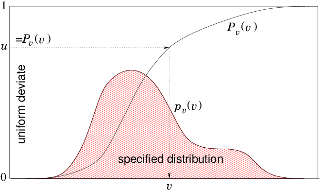
Fig.&nbsp;<a href="chap11.xml#Pselect">11.1</a> illustrates this process.
It is not always possible to invert the function analytically, but it
is always possible to do it numerically. One way is by root
finding<a 
id="root_finding_bisection112644"></a> e.g.&nbsp;bisection. 

<div class="p"><!----></div>
<a id="tth_fIg11.1">
</a>   <img src="figures/distribtransf.png" alt="figures/distribtransf.png" /><a id="distribtransf">
</a>
  
<div style="text-align:center">Figure 11.1: To obtain numerically a random variable <math xmlns="http://www.w3.org/1998/Math/MathML">
<mrow><mi>v</mi></mrow></math> with specified
    probability distribution <math xmlns="http://www.w3.org/1998/Math/MathML">
<mrow>
<msub><mrow><mi>p</mi></mrow><mrow><mi>v</mi></mrow>
</msub>
</mrow></math> (not to scale), calculate a table
    of the function <math xmlns="http://www.w3.org/1998/Math/MathML">
<mrow>
<msub><mrow><mi>P</mi></mrow><mrow><mi>v</mi></mrow>
</msub>
<mo stretchy="false">(</mo><mi>v</mi><mo stretchy="false">)</mo></mrow></math> by integration. Draw a random number from
    uniform deviate <math xmlns="http://www.w3.org/1998/Math/MathML">
<mrow><mi>u</mi></mrow></math>. Find the <math xmlns="http://www.w3.org/1998/Math/MathML">
<mrow><mi>v</mi></mrow></math> for which <math xmlns="http://www.w3.org/1998/Math/MathML">
<mrow>
<msub><mrow><mi>P</mi></mrow><mrow><mi>v</mi></mrow>
</msub>
<mo stretchy="false">(</mo><mi>v</mi><mo stretchy="false">)</mo><mo>=</mo><mi>u</mi></mrow></math> by
    interpolation. That's the random <math xmlns="http://www.w3.org/1998/Math/MathML">
<mrow><mi>v</mi></mrow></math>.<a id="Pselect">
</a></div>

<div class="p"><!----></div>
Since <math xmlns="http://www.w3.org/1998/Math/MathML">
<mrow>
<msub><mrow><mi>P</mi></mrow><mrow><mi>v</mi></mrow>
</msub>
</mrow></math> is monotonic, for any <math xmlns="http://www.w3.org/1998/Math/MathML">
<mrow><mi>u</mi></mrow></math> between 0 and 1, there is a
single root <math xmlns="http://www.w3.org/1998/Math/MathML">
<mrow><mi>v</mi></mrow></math> of the equation <math xmlns="http://www.w3.org/1998/Math/MathML">
<mrow>
<msub><mrow><mi>P</mi></mrow><mrow><mi>v</mi></mrow>
</msub>
<mo stretchy="false">(</mo><mi>v</mi><mo stretchy="false">)</mo><mo>-</mo><mi>u</mi><mo>=</mo><mn>0</mn></mrow></math>. Provided we can find that
root quickly, then given <math xmlns="http://www.w3.org/1998/Math/MathML">
<mrow><mi>u</mi></mrow></math> we can find <math xmlns="http://www.w3.org/1998/Math/MathML">
<mrow><mi>v</mi></mrow></math>. One way to make the root
finding quick is to generate a table of <math xmlns="http://www.w3.org/1998/Math/MathML">
<mrow>
<msub><mrow><mi>N</mi></mrow><mrow><mi>t</mi></mrow>
</msub>
</mrow></math> values of <math xmlns="http://www.w3.org/1998/Math/MathML">
<mrow><mi>v</mi></mrow></math> and <math xmlns="http://www.w3.org/1998/Math/MathML">
<mrow><mi>u</mi><mo>=</mo>
<msub><mrow><mi>P</mi></mrow><mrow><mi>v</mi></mrow>
</msub>
<mo stretchy="false">(</mo><mi>v</mi><mo stretchy="false">)</mo></mrow></math>,
equally spaced <em>in <math xmlns="http://www.w3.org/1998/Math/MathML">
<mrow><mi>u</mi></mrow></math></em> (not in <math xmlns="http://www.w3.org/1998/Math/MathML">
<mrow><mi>v</mi></mrow></math>). Then given any <math xmlns="http://www.w3.org/1998/Math/MathML">
<mrow><mi>u</mi></mrow></math>, the
index of the point just below <math xmlns="http://www.w3.org/1998/Math/MathML">
<mrow><mi>u</mi></mrow></math> is the integer value <math xmlns="http://www.w3.org/1998/Math/MathML">
<mrow><mi>i</mi><mo>=</mo></mrow></math> <math xmlns="http://www.w3.org/1998/Math/MathML">
<mrow><mi>u</mi></mrow></math>*<math xmlns="http://www.w3.org/1998/Math/MathML">
<mrow>
<msub><mrow><mi>N</mi></mrow><mrow><mi>t</mi></mrow>
</msub>
</mrow></math>,
and we can interpolate between it and the next point using the
fractional value of  <math xmlns="http://www.w3.org/1998/Math/MathML">
<mrow><mi>u</mi></mrow></math>*<math xmlns="http://www.w3.org/1998/Math/MathML">
<mrow>
<msub><mrow><mi>N</mi></mrow><mrow><mi>t</mi></mrow>
</msub>
</mrow></math>.<a href="footnote.xml#tthFtNtAHC" id="tthFrefAHC"><math xmlns="http://www.w3.org/1998/Math/MathML">
<mrow>
<msup><mrow></mrow><mrow><mn>72</mn></mrow>
</msup>
</mrow></math></a>

<div class="p"><!----></div>

<b>Rejection Method&nbsp;&nbsp;</b><a 
id="rejection_method112645"></a>
Another way of obtaining random values from some specified probability
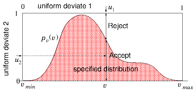
distribution is by the "Rejection Method", illustrated in Fig.&nbsp;<a href="chap11.xml#rejectionl">11.2</a>. This involves using a second random number to decide
whether or not to retain the first one chosen. The second random
number is used to weight the probability of the first one.
<div class="p"><!----></div>
<a id="tth_fIg11.2">
</a>     <img src="figures/rejection.png" alt="figures/rejection.png" /><a id="rejection">
</a>
    
<div style="text-align:center">Figure 11.2: The rejection method chooses a <math xmlns="http://www.w3.org/1998/Math/MathML">
<mrow><mi>v</mi></mrow></math> value randomly from a
      simple distribution (e.g.&nbsp;a constant) whose integral is
      invertible. Then a second random number decides whether it will
      be rejected or accepted. The fraction accepted at <math xmlns="http://www.w3.org/1998/Math/MathML">
<mrow><mi>v</mi></mrow></math> is equal
      to the ratio of <math xmlns="http://www.w3.org/1998/Math/MathML">
<mrow>
<msub><mrow><mi>p</mi></mrow><mrow><mi>v</mi></mrow>
</msub>
<mo stretchy="false">(</mo><mi>v</mi><mo stretchy="false">)</mo></mrow></math> to the simple invertible distribution.
      <math xmlns="http://www.w3.org/1998/Math/MathML">
<mrow>
<msub><mrow><mi>p</mi></mrow><mrow><mi>v</mi></mrow>
</msub>
<mo stretchy="false">(</mo><mi>v</mi><mo stretchy="false">)</mo></mrow></math> must be scaled by a constant factor to be everywhere
      less than the simple distribution (1 here).<a id="rejectionl">
</a></div>

<div class="p"><!----></div>
In effect this means picking points below the first scaled
distribution, in the illustrated case of a rectangular distribution,
uniformly distributed within the rectangle, and accepting only those
that are below <math xmlns="http://www.w3.org/1998/Math/MathML">
<mrow>
<msub><mrow><mi>p</mi></mrow><mrow><mi>v</mi></mrow>
</msub>
<mo stretchy="false">(</mo><mi>v</mi><mo stretchy="false">)</mo></mrow></math> (suitably scaled to be everywhere less than
1). Therefore some inefficiency is inevitable. If the area under
<math xmlns="http://www.w3.org/1998/Math/MathML">
<mrow>
<msub><mrow><mi>p</mi></mrow><mrow><mi>v</mi></mrow>
</msub>
<mo stretchy="false">(</mo><mi>v</mi><mo stretchy="false">)</mo></mrow></math> is, say, half the total, then twice as many total choices are
needed, and each requires two random numbers, giving four
<a 
id="efficiency_rejection_method112646"></a>times as many random numbers per
accepted point. Improvement on the second inefficiency can be obtained
by using a simply invertible function that fits <math xmlns="http://www.w3.org/1998/Math/MathML">
<mrow>
<msub><mrow><mi>p</mi></mrow><mrow><mi>v</mi></mrow>
</msub>
<mo stretchy="false">(</mo><mi>v</mi><mo stretchy="false">)</mo></mrow></math> more
closely. Even so, this will be slower than the tabulated function
method, unless the random number generator has very small cost.

<div class="p"><!----></div>

<b>Monte Carlo Integration&nbsp;&nbsp;</b> Notice by the way, that this
second<a 
id="Monte_Carlo_integration112647"></a> technique shows exactly how
"Monte Carlo Integration" can be done. Select points at random over
a line, or a rectangular area in two dimensions, or cuboid volume in
three dimensions. Decide whether each point is within the area/volume
of interest. If so, add the value of the function to be integrated to
the running total, if not, not. Repeat. At the end multiply the total
by the area/volume of the rectangle/cuboid divided by the number of
random points examined (total, not just those that are within the
area/volume).  That's the integral. Such a technique can be quite an
efficient way, and certainly an easy-to-program way, to integrate over
a volume for which it is simple to decide whether you are inside it
but hard to define systematically where the boundaries are. An example
might be the volume inside a cube but outside a sphere placed
off-center inside the cube. The method's drawback is that its accuracy
increases only like the inverse <em>square root</em> of the number of
points sampled. So if high accuracy is required, other methods may be
much more efficient.<a 
id="quasi-random_numbers112648"></a><a href="footnote.xml#tthFtNtAHD" id="tthFrefAHD"><math xmlns="http://www.w3.org/1998/Math/MathML">
<mrow>
<msup><mrow></mrow><mrow><mn>73</mn></mrow>
</msup>
</mrow></math></a>

<div class="p"><!----></div>
 <a id="tth_sEc11.3"></a><h2>
11.3&nbsp;&nbsp;Flux integration and injection choice.</h2>

<div class="p"><!----></div>
<a 
id="injection_particle113649"></a><a 
id="particle_injection113650"></a> Suppose we are
simulating a sub-volume that is embedded in a larger region. Particles
move in and out of the sub-volume. Something interesting is being
modelled within the subvolume, for example the interaction of some
object with the particles. If the volume is big enough, the region
outside the subvolume is relatively unaffected by the physics in the
subvolume, then we know or can specify what the distribution function
of particles is in the outer region, at the volume's boundaries. Assume
that periodic boundary conditions are not appropriate, because, for
example, they don't well represent an isolated interaction. How do we
determine statistically what particles to inject into the subvolume
across its boundary?
<div class="p"><!----></div>
<a id="tth_fIg11.3">
</a>     <img src="figures/injection.png" alt="figures/injection.png" /><a id="injection">
</a>
    
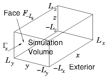
<div style="text-align:center">Figure 11.3: Simulating over a volume that is embedded in a wider
      external region, we need to be able to decide how to inject
      particles from the exterior into the simulation volume so as
      to represent statistically the exterior distribution.<a id="injcube">
</a></div>

<div class="p"><!----></div>
Suppose the volume is a cuboid shown in Fig.&nbsp;<a href="chap11.xml#injcube">11.3</a>. It has 6
faces, each of which is normal to one of the coordinate axes, and
located at <math xmlns="http://www.w3.org/1998/Math/MathML">
<mrow><mo>&PlusMinus;</mo>
<msub><mrow><mi>L</mi></mrow><mrow><mi>x</mi></mrow>
</msub>
</mrow></math>, <math xmlns="http://www.w3.org/1998/Math/MathML">
<mrow><mo>&PlusMinus;</mo>
<msub><mrow><mi>L</mi></mrow><mrow><mi>y</mi></mrow>
</msub>
</mrow></math> or <math xmlns="http://www.w3.org/1998/Math/MathML">
<mrow><mo>&PlusMinus;</mo>
<msub><mrow><mi>L</mi></mrow><mrow><mi>z</mi></mrow>
</msub>
</mrow></math>. We'll consider the face
perpendicular to <math xmlns="http://www.w3.org/1998/Math/MathML">
<mrow><mi>x</mi></mrow></math> which is at <math xmlns="http://www.w3.org/1998/Math/MathML">
<mrow><mo>-</mo>
<msub><mrow><mi>L</mi></mrow><mrow><mi>x</mi></mrow>
</msub>
</mrow></math>, so that positive velocity
<math xmlns="http://www.w3.org/1998/Math/MathML">
<mrow>
<msub><mrow><mi>v</mi></mrow><mrow><mi>x</mi></mrow>
</msub>
</mrow></math> corresponds to moving <em>into</em> the simulation sub-volume. We calculate
the rate at which particles are crossing the face into the
subvolume. If the distribution function is <math xmlns="http://www.w3.org/1998/Math/MathML">
<mrow><mi>f</mi><mo stretchy="false">(</mo><mi mathvariant="bold-italic">v</mi><mo>,</mo><mi mathvariant="bold-italic">x</mi><mo stretchy="false">)</mo></mrow></math>, then
the flux density<a 
id="flux_density113651"></a> in the <math xmlns="http://www.w3.org/1998/Math/MathML">
<mrow><mo>+</mo>
<msub><mrow><mi>v</mi></mrow><mrow><mi>x</mi></mrow>
</msub>
</mrow></math> direction is
<a id="fluxvxden">
</a><br />
<table width="100%"><tr><td align="center">
    <math xmlns="http://www.w3.org/1998/Math/MathML">
    <mstyle displaystyle="true"><mrow>
<msub><mrow><mi mathvariant="italic">&Gamma;</mi></mrow><mrow><mi>x</mi></mrow>
</msub>
<mo stretchy="false">(</mo><mi mathvariant="bold-italic">x</mi><mo stretchy="false">)</mo><mo>=</mo><mo>&int;</mo><mo>&int;</mo>
<msubsup><mrow><mo>&int;</mo></mrow><mrow>
<msub><mrow><mi>v</mi></mrow><mrow><mi>x</mi></mrow>
</msub>
<mo>=</mo><mn>0</mn> </mrow>
<mrow><mi mathvariant="italic">&infin;</mi></mrow></msubsup>

<msub><mrow><mi>v</mi></mrow><mrow><mi>x</mi></mrow>
</msub>
<mi>f</mi><mo stretchy="false">(</mo><mi mathvariant="bold-italic">v</mi><mo>,</mo><mi mathvariant="bold-italic">x</mi><mo stretchy="false">)</mo>
<msub><mrow><mi mathvariant="italic">dv</mi></mrow><mrow><mi>x</mi></mrow>
</msub>

<msub><mrow><mi mathvariant="italic">dv</mi></mrow><mrow><mi>y</mi></mrow>
</msub>

<msub><mrow><mi mathvariant="italic">dv</mi></mrow><mrow><mi>z</mi></mrow>
</msub>
<mi>&ensp;&ensp;</mi></mrow>
    </mstyle></math></td><td width="1">
    <math xmlns="http://www.w3.org/1998/Math/MathML">
    <mstyle displaystyle="true"><mrow><mo stretchy="false">(</mo><mn>11</mn><mo>.</mo><mn>13</mn><mo stretchy="false">)</mo></mrow>
    </mstyle></math>
</td></tr></table>


and the number entering across the face per unit time (the flux)<a 
id="flux113652"></a> is
<a id="fluxfac">
</a><br />
<table width="100%"><tr><td align="center">
    <math xmlns="http://www.w3.org/1998/Math/MathML">
    <mstyle displaystyle="true"><mrow>
<msub><mrow><mi>F</mi></mrow><mrow><mo>-</mo>
<msub><mrow><mi>L</mi></mrow><mrow><mi>x</mi></mrow>
</msub>
</mrow>
</msub>
<mo>=</mo>
<msubsup><mrow><mo>&int;</mo></mrow><mrow><mo>-</mo>
<msub><mrow><mi>L</mi></mrow><mrow><mi>y</mi></mrow>
</msub>
 </mrow>
<mrow>
<msub><mrow><mi>L</mi></mrow><mrow><mi>y</mi></mrow>
</msub>
</mrow></msubsup>

<msubsup><mrow><mo>&int;</mo></mrow><mrow><mo>-</mo>
<msub><mrow><mi>L</mi></mrow><mrow><mi>y</mi></mrow>
</msub>
 </mrow>
<mrow>
<msub><mrow><mi>L</mi></mrow><mrow><mi>y</mi></mrow>
</msub>
</mrow></msubsup>

<msub><mrow><mi mathvariant="italic">&Gamma;</mi></mrow><mrow><mi>x</mi></mrow>
</msub>
<mo stretchy="false">(</mo><mo>-</mo>
<msub><mrow><mi>L</mi></mrow><mrow><mi>x</mi></mrow>
</msub>
<mo>,</mo><mi>y</mi><mo>,</mo><mi>z</mi><mo stretchy="false">)</mo><mi>&ensp;&ensp;</mi><mi mathvariant="italic">dy</mi><mi mathvariant="italic">dz</mi><mo>.</mo></mrow>
    </mstyle></math></td><td width="1">
    <math xmlns="http://www.w3.org/1998/Math/MathML">
    <mstyle displaystyle="true"><mrow><mo stretchy="false">(</mo><mn>11</mn><mo>.</mo><mn>14</mn><mo stretchy="false">)</mo></mrow>
    </mstyle></math>
</td></tr></table>


<div class="p"><!----></div>
Assume that the outer region is steady, independent of time. We
proceed by evaluating the six fluxes <math xmlns="http://www.w3.org/1998/Math/MathML">
<mrow>
<msub><mrow><mi>F</mi></mrow><mrow><mi>j</mi></mrow>
</msub>
</mrow></math>, using the above
expressions and their equivalents for the six different faces.  At
each time step of the simulation, we decide how many particles to
inject into the subvolume from each face. The average number of
particles to inject in a timestep <math xmlns="http://www.w3.org/1998/Math/MathML">
<mrow><mi mathvariant="italic">&Delta;</mi><mi>t</mi></mrow></math> at face <math xmlns="http://www.w3.org/1998/Math/MathML">
<mrow><mi>j</mi></mrow></math> is equal to
<math xmlns="http://www.w3.org/1998/Math/MathML">
<mrow>
<msub><mrow><mi>F</mi></mrow><mrow><mi>j</mi></mrow>
</msub>
<mi mathvariant="italic">&Delta;</mi><mi>t</mi></mrow></math>. If this number is large,<a href="footnote.xml#tthFtNtAHE" id="tthFrefAHE"><math xmlns="http://www.w3.org/1998/Math/MathML">
<mrow>
<msup><mrow></mrow><mrow><mn>74</mn></mrow>
</msup>
</mrow></math></a> then it may
be appropriate to inject just that number (although dealing with the
non-integer fractional part of the number needs consideration). But if
it is of order unity or even smaller, then that does not correctly
represent the statistics. In that case we need to decide statistically
at each step how many particles are injected: 0,1,2 ...

<div class="p"><!----></div>
It is a standard result of probability theory <a href="footnote.xml#tthFtNtAHF" id="tthFrefAHF"><math xmlns="http://www.w3.org/1998/Math/MathML">
<mrow>
<msup><mrow></mrow><mrow><mn>75</mn></mrow>
</msup>
</mrow></math></a> that
if events (in this case injections) take place randomly and
uncorrelated with each other at a fixed average rate <math xmlns="http://www.w3.org/1998/Math/MathML">
<mrow><mi>r</mi></mrow></math> (per sample,
in this case per time-step) then the number <math xmlns="http://www.w3.org/1998/Math/MathML">
<mrow><mi>n</mi></mrow></math> that happens in any
particular sample is an integer random variable with "Poisson
distribution"<a 
id="Poisson_distribution113653"></a>: a discrete probability distribution
<a id="PoissonDist">
</a><br />
<table width="100%"><tr><td align="center">
    <math xmlns="http://www.w3.org/1998/Math/MathML">
    <mstyle displaystyle="true"><mrow>
<msub><mrow><mi>p</mi></mrow><mrow><mi>n</mi></mrow>
</msub>
<mo>=</mo><mi>exp</mi><mo stretchy="false">(</mo><mo>-</mo><mi>r</mi><mo stretchy="false">)</mo>
<msup><mrow><mi>r</mi></mrow><mrow><mi>n</mi></mrow>
</msup>
<mo stretchy="false">/</mo><mi>n</mi><mo>!</mo><mi>&ensp;</mi><mo>.</mo></mrow>
    </mstyle></math></td><td width="1">
    <math xmlns="http://www.w3.org/1998/Math/MathML">
    <mstyle displaystyle="true"><mrow><mo stretchy="false">(</mo><mn>11</mn><mo>.</mo><mn>15</mn><mo stretchy="false">)</mo></mrow>
    </mstyle></math>
</td></tr></table>


The parameter giving the rate, <math xmlns="http://www.w3.org/1998/Math/MathML">
<mrow><mi>r</mi></mrow></math>, is a real number, but the number
for each sample, <math xmlns="http://www.w3.org/1998/Math/MathML">
<mrow><mi>n</mi></mrow></math>, is an integer.  One can rapidly verify that,
since <math xmlns="http://www.w3.org/1998/Math/MathML">
<mrow>
<munderover><mo>&sum;</mo><mrow><mi>n</mi><mo>=</mo><mn>0</mn> </mrow>
<mrow><mi mathvariant="italic">&infin;</mi></mrow></munderover>
<msup><mrow><mi>r</mi></mrow><mrow><mi>n</mi></mrow>
</msup>
<mo stretchy="false">/</mo><mi>n</mi><mo>!</mo><mo>=</mo><mi>exp</mi><mo stretchy="false">(</mo><mi>r</mi><mo stretchy="false">)</mo></mrow></math>, the probabilities are
properly normalized: <math xmlns="http://www.w3.org/1998/Math/MathML">
<mrow>
<munder><mo>&sum;</mo><mrow><mi>n</mi></mrow>
</munder>

<msub><mrow><mi>p</mi></mrow><mrow><mi>n</mi></mrow>
</msub>
<mo>=</mo><mn>1</mn></mrow></math>.  The mean rate is <math xmlns="http://www.w3.org/1998/Math/MathML">
<mrow>
<munder><mo>&sum;</mo><mrow><mi>n</mi></mrow>
</munder>

<msub><mrow><mi mathvariant="italic">np</mi></mrow><mrow><mi>n</mi></mrow>
</msub>
<mo>=</mo><mi>r</mi></mrow></math>
(as advertized). The variance, it turns out, is also <math xmlns="http://www.w3.org/1998/Math/MathML">
<mrow><mi>r</mi></mrow></math>. So the
standard deviation is <math xmlns="http://www.w3.org/1998/Math/MathML">
<mrow><msqrt><mrow><mi>r</mi></mrow></msqrt></mrow></math>. The value <math xmlns="http://www.w3.org/1998/Math/MathML">
<mrow>
<msub><mrow><mi>p</mi></mrow><mrow><mi>n</mi></mrow>
</msub>
</mrow></math> gives us precisely
the probability that <math xmlns="http://www.w3.org/1998/Math/MathML">
<mrow><mi>n</mi></mrow></math> particles will need to be injected when the
flux is <math xmlns="http://www.w3.org/1998/Math/MathML">
<mrow><mi>r</mi><mo>=</mo>
<msub><mrow><mi>F</mi></mrow><mrow><mi>j</mi></mrow>
</msub>
</mrow></math>. So the first step in deciding injections is to select
randomly a number to be injected, from the Poisson distribution eq.&nbsp;(<a href="chap11.xml#PoissonDist">11.15</a>). There are various ways to do this (including
library routines). The root-finding approach is easily applied,
because the cumulative probability function <math xmlns="http://www.w3.org/1998/Math/MathML">
<mrow>
<msub><mrow><mi>P</mi></mrow><mrow><mi>u</mi></mrow>
</msub>
<mo stretchy="false">(</mo><mi>u</mi><mo stretchy="false">)</mo></mrow></math> can be considered
to consist of steps of height <math xmlns="http://www.w3.org/1998/Math/MathML">
<mrow>
<msub><mrow><mi>p</mi></mrow><mrow><mi>n</mi></mrow>
</msub>
</mrow></math> at the integers <math xmlns="http://www.w3.org/1998/Math/MathML">
<mrow><mi>n</mi></mrow></math> (and constant
in between).

<div class="p"><!----></div>
Next we need to decide where on the surface each injection is going to
take place. If the flux density is uniform, then we just pick randomly
a position corresponding to <math xmlns="http://www.w3.org/1998/Math/MathML">
<mrow><mo>-</mo>
<msub><mrow><mi>L</mi></mrow><mrow><mi>y</mi></mrow>
</msub>
<mo>&le;</mo><mi>y</mi><mo>&le;</mo>
<msub><mrow><mi>L</mi></mrow><mrow><mi>y</mi></mrow>
</msub>
</mrow></math> and <math xmlns="http://www.w3.org/1998/Math/MathML">
<mrow><mo>-</mo>
<msub><mrow><mi>L</mi></mrow><mrow><mi>z</mi></mrow>
</msub>
<mo>&le;</mo><mi>z</mi><mo>&le;</mo>
<msub><mrow><mi>L</mi></mrow><mrow><mi>z</mi></mrow>
</msub>
</mrow></math>. Non-uniform flux density, however, introduces another distribution
function inversion headache. It's more work, but straightforward. 

<div class="p"><!----></div>
Finally we need to select the actual velocity of the particle. Very
importantly, the probability distribution of this selection is
<em>not</em> just the velocity distribution function, or the velocity
distribution function restricted to positive <math xmlns="http://www.w3.org/1998/Math/MathML">
<mrow>
<msub><mrow><mi>v</mi></mrow><mrow><mi>x</mi></mrow>
</msub>
</mrow></math>. No, it it the
<em>flux</em> distribution <math xmlns="http://www.w3.org/1998/Math/MathML">
<mrow>
<msub><mrow><mi>v</mi></mrow><mrow><mi>x</mi></mrow>
</msub>
<mi>f</mi><mo stretchy="false">(</mo><mi mathvariant="bold-italic">v</mi><mo>,</mo><mi mathvariant="bold-italic">x</mi><mo stretchy="false">)</mo></mrow></math> weighted by the
normal velocity <math xmlns="http://www.w3.org/1998/Math/MathML">
<mrow>
<msub><mrow><mi>v</mi></mrow><mrow><mi>x</mi></mrow>
</msub>
</mrow></math> (for an <math xmlns="http://www.w3.org/1998/Math/MathML">
<mrow><mi>x</mi></mrow></math>-surface) if positive (otherwise
zero). If the distribution is separable,
<math xmlns="http://www.w3.org/1998/Math/MathML">
<mrow><mi>f</mi><mo stretchy="false">(</mo><mi mathvariant="bold-italic">v</mi><mo stretchy="false">)</mo><mo>=</mo>
<msub><mrow><mi>f</mi></mrow><mrow><mi>x</mi></mrow>
</msub>
<mo stretchy="false">(</mo>
<msub><mrow><mi>v</mi></mrow><mrow><mi>x</mi></mrow>
</msub>
<mo stretchy="false">)</mo>
<msub><mrow><mi>f</mi></mrow><mrow><mi>y</mi></mrow>
</msub>
<mo stretchy="false">(</mo>
<msub><mrow><mi>v</mi></mrow><mrow><mi>y</mi></mrow>
</msub>
<mo stretchy="false">)</mo>
<msub><mrow><mi>f</mi></mrow><mrow><mi>z</mi></mrow>
</msub>
<mo stretchy="false">(</mo>
<msub><mrow><mi>v</mi></mrow><mrow><mi>z</mi></mrow>
</msub>
<mo stretchy="false">)</mo></mrow></math>, as it is if it is Maxwellian,
then the tangential velocities <math xmlns="http://www.w3.org/1998/Math/MathML">
<mrow>
<msub><mrow><mi>v</mi></mrow><mrow><mi>y</mi></mrow>
</msub>
</mrow></math>, <math xmlns="http://www.w3.org/1998/Math/MathML">
<mrow>
<msub><mrow><mi>v</mi></mrow><mrow><mi>z</mi></mrow>
</msub>
</mrow></math>, can be treated
separately: select two different velocities from the respective
distributions. And select <math xmlns="http://www.w3.org/1998/Math/MathML">
<mrow>
<msub><mrow><mi>v</mi></mrow><mrow><mi>x</mi></mrow>
</msub>
</mrow></math> (positive) from a probability
distribution proportional to <math xmlns="http://www.w3.org/1998/Math/MathML">
<mrow>
<msub><mrow><mi>v</mi></mrow><mrow><mi>x</mi></mrow>
</msub>

<msub><mrow><mi>f</mi></mrow><mrow><mi>x</mi></mrow>
</msub>
<mo stretchy="false">(</mo>
<msub><mrow><mi>v</mi></mrow><mrow><mi>x</mi></mrow>
</msub>
<mo stretchy="false">)</mo></mrow></math>.

<div class="p"><!----></div>
If <math xmlns="http://www.w3.org/1998/Math/MathML">
<mrow><mi>f</mi></mrow></math> is not separable, then a more elaborate random selection is
required. Suppose we have the cumulative probability distribution of
velocities <math xmlns="http://www.w3.org/1998/Math/MathML">
<mrow><mi>P</mi><mo stretchy="false">(</mo>
<msub><mrow><mi>v</mi></mrow><mrow><mi>x</mi></mrow>
</msub>
<mo>,</mo>
<msub><mrow><mi>v</mi></mrow><mrow><mi>y</mi></mrow>
</msub>
<mo>,</mo>
<msub><mrow><mi>v</mi></mrow><mrow><mi>z</mi></mrow>
</msub>
<mo stretchy="false">)</mo></mrow></math> for all interesting values of
velocity. Notice that if <math xmlns="http://www.w3.org/1998/Math/MathML">
<mrow>
<msub><mrow><mi>v</mi></mrow><mrow><mi mathvariant="italic">xmax</mi></mrow>
</msub>
</mrow></math>, <math xmlns="http://www.w3.org/1998/Math/MathML">
<mrow>
<msub><mrow><mi>v</mi></mrow><mrow><mi mathvariant="italic">ymax</mi></mrow>
</msub>
</mrow></math>, <math xmlns="http://www.w3.org/1998/Math/MathML">
<mrow>
<msub><mrow><mi>v</mi></mrow><mrow><mi mathvariant="italic">zmax</mi></mrow>
</msub>
</mrow></math> denote the
largest relevant values of <math xmlns="http://www.w3.org/1998/Math/MathML">
<mrow>
<msub><mrow><mi>v</mi></mrow><mrow><mi>x</mi></mrow>
</msub>
</mrow></math>, <math xmlns="http://www.w3.org/1998/Math/MathML">
<mrow>
<msub><mrow><mi>v</mi></mrow><mrow><mi>y</mi></mrow>
</msub>
</mrow></math> and <math xmlns="http://www.w3.org/1998/Math/MathML">
<mrow>
<msub><mrow><mi>v</mi></mrow><mrow><mi>z</mi></mrow>
</msub>
</mrow></math>, beyond which <math xmlns="http://www.w3.org/1998/Math/MathML">
<mrow><mi>f</mi><mo>=</mo><mn>0</mn></mrow></math>,
then <math xmlns="http://www.w3.org/1998/Math/MathML">
<mrow><mi>P</mi><mo stretchy="false">(</mo>
<msub><mrow><mi>v</mi></mrow><mrow><mi>x</mi></mrow>
</msub>
<mo>,</mo>
<msub><mrow><mi>v</mi></mrow><mrow><mi mathvariant="italic">ymax</mi></mrow>
</msub>
<mo>,</mo>
<msub><mrow><mi>v</mi></mrow><mrow><mi mathvariant="italic">zmax</mi></mrow>
</msub>
<mo stretchy="false">)</mo></mrow></math> is a function of just one variable
<math xmlns="http://www.w3.org/1998/Math/MathML">
<mrow>
<msub><mrow><mi>v</mi></mrow><mrow><mi>x</mi></mrow>
</msub>
</mrow></math>, and is the cumulative probability distribution integrated over
the entire relevant range of the other velocity components. That is,
it is the one-dimensional cumulative probability distribution of
<math xmlns="http://www.w3.org/1998/Math/MathML">
<mrow>
<msub><mrow><mi>v</mi></mrow><mrow><mi>x</mi></mrow>
</msub>
</mrow></math>. We can convert it into a 
one-dimensional<a 
id="cumulative_flux_probability113654"></a> 
flux cumulative probability by performing the following
integral (numerically, discretely).
<a id="fluxinteg">
</a><br />
<table width="100%"><tr><td align="center">
    <math xmlns="http://www.w3.org/1998/Math/MathML">
    <mstyle displaystyle="true"><mrow>
<mtable displaystyle="true" align="right" width="80%">
<mtr><mtd columnalign="right" columnspan="1"><mrow><mi>F</mi><mo stretchy="false">(</mo>
<msub><mrow><mi>v</mi></mrow><mrow><mi>x</mi></mrow>
</msub>
<mo stretchy="false">)</mo></mrow>
</mtd><mtd columnalign="left">
<mrow><mo>=</mo></mrow>
</mtd><mtd columnalign="left">
<mrow>
<msubsup><mrow><mo>&int;</mo></mrow><mrow><mn>0</mn> </mrow>
<mrow>
<msub><mrow><mi>v</mi></mrow><mrow><mi>x</mi></mrow>
</msub>
</mrow></msubsup>

<msub><mrow><mi>v</mi></mrow><mrow><mi>x</mi></mrow>
</msub>
<mo>'</mo>
<mfrac><mrow><mo>&part;</mo></mrow>
<mrow><mo>&part;</mo>
<msub><mrow><mi>v</mi></mrow><mrow><mi>x</mi></mrow>
</msub>
<mo>'</mo></mrow>
</mfrac>
<mi>P</mi><mo stretchy="false">(</mo>
<msub><mrow><mi>v</mi></mrow><mrow><mi>x</mi></mrow>
</msub>
<mo>'</mo><mo>,</mo>
<msub><mrow><mi>v</mi></mrow><mrow><mi mathvariant="italic">ymax</mi></mrow>
</msub>
<mo>,</mo>
<msub><mrow><mi>v</mi></mrow><mrow><mi mathvariant="italic">zmax</mi></mrow>
</msub>
<mo stretchy="false">)</mo><mi>&ensp;&ensp;</mi>
<msub><mrow><mi mathvariant="italic">dv</mi></mrow><mrow><mi>x</mi></mrow>
</msub>
<mo>'</mo></mrow>
</mtd><mtd columnalign="right">&emsp;&emsp;&emsp;&emsp;&emsp;&emsp;<mo stretchy="false">(</mo><mn>11</mn><mo>.</mo><mn>16</mn><mo stretchy="false">)</mo></mtd></mtr>
<mtr><mtd columnalign="right" columnspan="1"><mrow></mrow>
</mtd><mtd columnalign="left">
<mrow><mo>=</mo></mrow>
</mtd><mtd columnalign="left">
<mrow>
<msub><mrow><mi>v</mi></mrow><mrow><mi>x</mi></mrow>
</msub>
<mi>P</mi><mo stretchy="false">(</mo>
<msub><mrow><mi>v</mi></mrow><mrow><mi>x</mi></mrow>
</msub>
<mo>,</mo>
<msub><mrow><mi>v</mi></mrow><mrow><mi mathvariant="italic">ymax</mi></mrow>
</msub>
<mo>,</mo>
<msub><mrow><mi>v</mi></mrow><mrow><mi mathvariant="italic">zmax</mi></mrow>
</msub>
<mo stretchy="false">)</mo><mo>-</mo>
<msubsup><mrow><mo>&int;</mo></mrow><mrow><mn>0</mn> </mrow>
<mrow>
<msub><mrow><mi>v</mi></mrow><mrow><mi>x</mi></mrow>
</msub>
</mrow></msubsup>
<mi>P</mi><mo stretchy="false">(</mo>
<msub><mrow><mi>v</mi></mrow><mrow><mi>x</mi></mrow>
</msub>
<mo>'</mo><mo>,</mo>
<msub><mrow><mi>v</mi></mrow><mrow><mi mathvariant="italic">ymax</mi></mrow>
</msub>
<mo>,</mo>
<msub><mrow><mi>v</mi></mrow><mrow><mi mathvariant="italic">zmax</mi></mrow>
</msub>
<mo stretchy="false">)</mo><mi>&ensp;&ensp;</mi>
<msub><mrow><mi mathvariant="italic">dv</mi></mrow><mrow><mi>x</mi></mrow>
</msub>
<mo>'</mo><mo>.</mo></mrow>
</mtd></mtr>
</mtable>
</mrow>
    </mstyle></math>
</td></tr></table>
<br />

Afterwards, we can normalize <math xmlns="http://www.w3.org/1998/Math/MathML">
<mrow><mi>F</mi><mo stretchy="false">(</mo>
<msub><mrow><mi>v</mi></mrow><mrow><mi>x</mi></mrow>
</msub>
<mo stretchy="false">)</mo></mrow></math> by dividing by <math xmlns="http://www.w3.org/1998/Math/MathML">
<mrow><mi>F</mi><mo stretchy="false">(</mo>
<msub><mrow><mi>v</mi></mrow><mrow><mi mathvariant="italic">xmax</mi></mrow>
</msub>
<mo stretchy="false">)</mo></mrow></math>,
ariving at the cumulative flux weighted probability for <math xmlns="http://www.w3.org/1998/Math/MathML">
<mrow>
<msub><mrow><mi>v</mi></mrow><mrow><mi>x</mi></mrow>
</msub>
</mrow></math>.

<div class="p"><!----></div>
We then proceed as follows. 

<div class="p"><!----></div>
<br />
<table>
<tr><td align="left">1.</td><td width="0">Choose a random <math xmlns="http://www.w3.org/1998/Math/MathML">
<mrow>
<msub><mrow><mi>v</mi></mrow><mrow><mi>x</mi></mrow>
</msub>
</mrow></math> from its cumulative flux-weighted probability
  <math xmlns="http://www.w3.org/1998/Math/MathML">
<mrow><mi>F</mi><mo stretchy="false">(</mo>
<msub><mrow><mi>v</mi></mrow><mrow><mi>x</mi></mrow>
</msub>
<mo stretchy="false">)</mo></mrow></math>.</td></tr>
<tr><td align="left">2.</td><td width="0">Choose a random <math xmlns="http://www.w3.org/1998/Math/MathML">
<mrow>
<msub><mrow><mi>v</mi></mrow><mrow><mi>y</mi></mrow>
</msub>
</mrow></math> from its cumulative probability for the
  already chosen <math xmlns="http://www.w3.org/1998/Math/MathML">
<mrow>
<msub><mrow><mi>v</mi></mrow><mrow><mi>x</mi></mrow>
</msub>
</mrow></math>, namely <math xmlns="http://www.w3.org/1998/Math/MathML">
<mrow><mi>P</mi><mo stretchy="false">(</mo>
<msub><mrow><mi>v</mi></mrow><mrow><mi>x</mi></mrow>
</msub>
<mo>,</mo>
<msub><mrow><mi>v</mi></mrow><mrow><mi>y</mi></mrow>
</msub>
<mo>,</mo>
<msub><mrow><mi>v</mi></mrow><mrow><mi mathvariant="italic">zmax</mi></mrow>
</msub>
<mo stretchy="false">)</mo></mrow></math> regarded as a
  function only of <math xmlns="http://www.w3.org/1998/Math/MathML">
<mrow>
<msub><mrow><mi>v</mi></mrow><mrow><mi>y</mi></mrow>
</msub>
</mrow></math>.</td></tr>
<tr><td align="left">3.</td><td width="0">Choose a random <math xmlns="http://www.w3.org/1998/Math/MathML">
<mrow>
<msub><mrow><mi>v</mi></mrow><mrow><mi>z</mi></mrow>
</msub>
</mrow></math> from its cumulative probability for the
  already chosen <math xmlns="http://www.w3.org/1998/Math/MathML">
<mrow>
<msub><mrow><mi>v</mi></mrow><mrow><mi>x</mi></mrow>
</msub>
</mrow></math> and <math xmlns="http://www.w3.org/1998/Math/MathML">
<mrow>
<msub><mrow><mi>v</mi></mrow><mrow><mi>y</mi></mrow>
</msub>
</mrow></math>, namely <math xmlns="http://www.w3.org/1998/Math/MathML">
<mrow><mi>P</mi><mo stretchy="false">(</mo>
<msub><mrow><mi>v</mi></mrow><mrow><mi>x</mi></mrow>
</msub>
<mo>,</mo>
<msub><mrow><mi>v</mi></mrow><mrow><mi>y</mi></mrow>
</msub>
<mo>,</mo>
<msub><mrow><mi>v</mi></mrow><mrow><mi>z</mi></mrow>
</msub>
<mo stretchy="false">)</mo></mrow></math> regarded as a
  function only of <math xmlns="http://www.w3.org/1998/Math/MathML">
<mrow>
<msub><mrow><mi>v</mi></mrow><mrow><mi>z</mi></mrow>
</msub>
</mrow></math>.</td></tr></table>


<div class="p"><!----></div>
<br /> Naturally for other faces, <math xmlns="http://www.w3.org/1998/Math/MathML">
<mrow><mi>y</mi></mrow></math> and <math xmlns="http://www.w3.org/1998/Math/MathML">
<mrow><mi>z</mi></mrow></math> one has to
start with the corresponding velocity component and cycle round the
indices.  For steady external conditions all the cumulative velocity
probabilities need to be calculated only once, and then
stored for subsequent time steps.

<div class="p"><!----></div>

<b>Discrete particle representation&nbsp;&nbsp;</b> An alternative to this
continuum approach is to suppose that the external distribution
function is represented by a perhaps large number, <math xmlns="http://www.w3.org/1998/Math/MathML">
<mrow><mi>N</mi></mrow></math>, (maybe
millions) of representative "particles" distributed in accordance
with the external velocity distribution function. Particle <math xmlns="http://www.w3.org/1998/Math/MathML">
<mrow><mi>k</mi></mrow></math> has
velocity <math xmlns="http://www.w3.org/1998/Math/MathML">
<mrow>
<msub><mrow><mi mathvariant="bold-italic">v</mi></mrow><mrow><mi>k</mi></mrow>
</msub>
</mrow></math> and the density of particles in phase space is
proportional to the distribution function, that is to the probability
distribution. Then if we wished to select randomly a velocity from the
particle distribution we simply arrange the particles in order and
pick one of them at random. However, when we want the particles to be
flux-weighted, in normal direction <math xmlns="http://www.w3.org/1998/Math/MathML">
<mrow>
<mover><mrow><mi mathvariant="bold-italic">n</mi></mrow>
<mo>&Hat;</mo></mover>
</mrow></math> say, we must select
them with probability proportional to <math xmlns="http://www.w3.org/1998/Math/MathML">
<mrow>
<msub><mrow><mi>v</mi></mrow><mrow><mi>n</mi></mrow>
</msub>
<mo>=</mo>
<mover><mrow><mi mathvariant="bold-italic">n</mi></mrow>
<mo>&Hat;</mo></mover>
<mo>.</mo><mi mathvariant="bold-italic">v</mi></mrow></math> (when
positive, and zero when negative). Therefore, for this normal
direction we must consider each particle to have appropriate weight.
We associate each particle with a real<a href="footnote.xml#tthFtNtAHG" id="tthFrefAHG"><math xmlns="http://www.w3.org/1998/Math/MathML">
<mrow>
<msup><mrow></mrow><mrow><mn>76</mn></mrow>
</msup>
</mrow></math></a> index <math xmlns="http://www.w3.org/1998/Math/MathML">
<mrow><mi>r</mi></mrow></math> so that when <math xmlns="http://www.w3.org/1998/Math/MathML">
<mrow>
<msub><mrow><mi>r</mi></mrow><mrow><mi>k</mi></mrow>
</msub>
<mo>&le;</mo><mi>r</mi><mo>&lt;</mo>
<msub><mrow><mi>r</mi></mrow><mrow><mi>k</mi><mo>+</mo><mn>1</mn></mrow>
</msub>
</mrow></math> the particle <math xmlns="http://www.w3.org/1998/Math/MathML">
<mrow><mi>k</mi></mrow></math> is indicated. The interval length
allocated to particle <math xmlns="http://www.w3.org/1998/Math/MathML">
<mrow><mi>k</mi></mrow></math> is chosen proportional to its weight, so
that <math xmlns="http://www.w3.org/1998/Math/MathML">
<mrow>
<msub><mrow><mi>r</mi></mrow><mrow><mi>k</mi><mo>+</mo><mn>1</mn></mrow>
</msub>
<mo>-</mo>
<msub><mrow><mi>r</mi></mrow><mrow><mi>k</mi></mrow>
</msub>
<mo>&prop;</mo>
<mover><mrow><mi mathvariant="bold-italic">n</mi></mrow>
<mo>&Hat;</mo></mover>
<mo>.</mo>
<msub><mrow><mi mathvariant="bold-italic">v</mi></mrow><mrow><mi>k</mi></mrow>
</msub>
</mrow></math>. Then the
selection consists of a random number draw <math xmlns="http://www.w3.org/1998/Math/MathML">
<mrow><mi>x</mi></mrow></math>, multiplied by the
total real index range and indexed to the particle and hence to its
velocity: <math xmlns="http://www.w3.org/1998/Math/MathML">
<mrow><mi>x</mi><mo stretchy="false">(</mo>
<msub><mrow><mi>r</mi></mrow><mrow><mi>N</mi><mo>+</mo><mn>1</mn></mrow>
</msub>
<mo>-</mo>
<msub><mrow><mi>r</mi></mrow><mrow><mn>1</mn></mrow>
</msub>
<mo stretchy="false">)</mo><mo>+</mo>
<msub><mrow><mi>r</mi></mrow><mrow><mn>1</mn></mrow>
</msub>
<mo>=</mo><mi>r</mi><mo>&rarr;</mo><mi>k</mi><mo>&rarr;</mo>
<msub><mrow><mi mathvariant="bold-italic">v</mi></mrow><mrow><mi>k</mi></mrow>
</msub>
</mrow></math>. The discreteness
of the particle distribution will generally not be an important
limitation for a process that already relies on random particle
representation. The position of injection will anyway be selected
differently even if a representative particle velocity is selected
more than once.

<div class="p"><!----></div>

<h2>Worked example: High Dimensionality Integration</h2>

<div class="p"><!----></div>
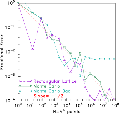
Monte Carlo techniques are commonly used for high-dimensional
<a 
id="high-dimensionality113655"></a><a 
id="dimensionality113656"></a>problems; integration
is perhaps the simplest example.<a 
id="Monte_Carlo_integration113657"></a> The
reasoning is approximately this. When there are <math xmlns="http://www.w3.org/1998/Math/MathML">
<mrow><mi>d</mi></mrow></math> dimensions, the
total number of points in a grid whose size is <math xmlns="http://www.w3.org/1998/Math/MathML">
<mrow><mi>M</mi></mrow></math> in each
coordinate-direction is <math xmlns="http://www.w3.org/1998/Math/MathML">
<mrow><mi>N</mi><mo>=</mo>
<msup><mrow><mi>M</mi></mrow><mrow><mi>d</mi></mrow>
</msup>
</mrow></math>. The fractional uncertainty in
estimating a one-dimensional integral of a function with only isolated
discontinuities, based upon evaluating it at <math xmlns="http://www.w3.org/1998/Math/MathML">
<mrow><mi>M</mi></mrow></math> grid points, may be
estimated as <math xmlns="http://www.w3.org/1998/Math/MathML">
<mrow><mo>&prop;</mo><mn>1</mn><mo stretchy="false">/</mo><mi>M</mi></mrow></math>. If this estimate still applies to multiple
dimension integration (and this is the dubious part), then the
fractional uncertainty is <math xmlns="http://www.w3.org/1998/Math/MathML">
<mrow><mo>&prop;</mo>
<mfrac><mrow><mn>1</mn></mrow>
<mrow><mi>M</mi></mrow>
</mfrac>
<mo>=</mo>
<msup><mrow><mi>N</mi></mrow><mrow><mo>-</mo><mn>1</mn><mo stretchy="false">/</mo><mi>d</mi></mrow>
</msup>
</mrow></math>. By
comparison, the uncertainty in a Monte-Carlo estimate of the integral
based on <math xmlns="http://www.w3.org/1998/Math/MathML">
<mrow><mi>N</mi></mrow></math> evaluations is <math xmlns="http://www.w3.org/1998/Math/MathML">
<mrow><mo>&prop;</mo>
<msup><mrow><mi>N</mi></mrow><mrow><mo>-</mo><mn>1</mn><mo stretchy="false">/</mo><mn>2</mn></mrow>
</msup>
</mrow></math>. When <math xmlns="http://www.w3.org/1998/Math/MathML">
<mrow><mi>d</mi></mrow></math> is larger
than 2, the Monte Carlo square-root convergence scaling is better than
the grid estimate. And if <math xmlns="http://www.w3.org/1998/Math/MathML">
<mrow><mi>d</mi></mrow></math> is very large, Monte Carlo is much
better.  Is this argument correct?  Test it by obtaining the volume of
a four-dimensional hypersphere<a 
id="hypersphere113658"></a> by numerical
integration, comparing a grid technique with Monte Carlo. 
<div class="p"><!----></div>
<br />A four-dimensional sphere of radius 1 consists of all those points for
which <math xmlns="http://www.w3.org/1998/Math/MathML">
<mrow>
<msup><mrow><mi>r</mi></mrow><mrow><mn>2</mn></mrow>
</msup>
<mo>=</mo>
<msubsup><mrow><mi>x</mi></mrow><mrow><mn>1</mn> </mrow>
<mrow><mn>2</mn></mrow></msubsup>
<mo>+</mo>
<msubsup><mrow><mi>x</mi></mrow><mrow><mn>2</mn> </mrow>
<mrow><mn>2</mn></mrow></msubsup>
<mo>+</mo>
<msubsup><mrow><mi>x</mi></mrow><mrow><mn>3</mn> </mrow>
<mrow><mn>2</mn></mrow></msubsup>
<mo>+</mo>
<msubsup><mrow><mi>x</mi></mrow><mrow><mn>4</mn> </mrow>
<mrow><mn>2</mn></mrow></msubsup>
<mo>&le;</mo><mn>1</mn></mrow></math>. Its volume is known
analytically; it is <math xmlns="http://www.w3.org/1998/Math/MathML">
<mrow>
<msup><mrow><mi mathvariant="italic">&pi;</mi></mrow><mrow><mn>2</mn></mrow>
</msup>
<mo stretchy="false">/</mo><mn>2</mn></mrow></math>. Let us evaluate the volume numerically
by examing the unit hypercube <math xmlns="http://www.w3.org/1998/Math/MathML">
<mrow><mn>0</mn><mo>&le;</mo>
<msub><mrow><mi>x</mi></mrow><mrow><mi>i</mi></mrow>
</msub>
<mo>&le;</mo><mn>1</mn></mrow></math>, <math xmlns="http://www.w3.org/1998/Math/MathML">
<mrow><mi>i</mi><mo>=</mo><mn>1</mn><mo>,</mo><mo>&#x2026;</mo><mo>,</mo><mn>4</mn></mrow></math>. It is
<math xmlns="http://www.w3.org/1998/Math/MathML">
<mrow><mn>1</mn><mo stretchy="false">/</mo>
<msup><mrow><mn>2</mn></mrow><mrow><mn>4</mn></mrow>
</msup>
<mo>=</mo><mn>1</mn><mo stretchy="false">/</mo><mn>16</mn></mrow></math>th of the hypercube <math xmlns="http://www.w3.org/1998/Math/MathML">
<mrow><mo>-</mo><mn>1</mn><mo>&le;</mo>
<msub><mrow><mi>x</mi></mrow><mrow><mi>i</mi></mrow>
</msub>
<mo>&le;</mo><mn>1</mn></mrow></math>, inside of which the
hypersphere fits; so the volume of of the hypersphere that lies
within the <math xmlns="http://www.w3.org/1998/Math/MathML">
<mrow><mn>0</mn><mo>&le;</mo>
<msub><mrow><mi>x</mi></mrow><mrow><mi>i</mi></mrow>
</msub>
<mo>&le;</mo><mn>1</mn></mrow></math> unit hypercube is <math xmlns="http://www.w3.org/1998/Math/MathML">
<mrow><mn>1</mn><mo stretchy="false">/</mo><mn>16</mn></mrow></math>th of its total
volume; it is <math xmlns="http://www.w3.org/1998/Math/MathML">
<mrow>
<msup><mrow><mi mathvariant="italic">&pi;</mi></mrow><mrow><mn>2</mn></mrow>
</msup>
<mo stretchy="false">/</mo><mn>32</mn></mrow></math>. We calculate this volume numerically by discrete
integration as follows.

<div class="p"><!----></div>
A deterministic (non-random) integration of the volume consists of
constructing an equally spaced lattice<a 
id="lattice113659"></a> of points at the
center of cells that fill the unit cube. If there are <math xmlns="http://www.w3.org/1998/Math/MathML">
<mrow><mi>M</mi></mrow></math> points per
edge, then the lattice positions in the dimension <math xmlns="http://www.w3.org/1998/Math/MathML">
<mrow><mi>i</mi></mrow></math> (<math xmlns="http://www.w3.org/1998/Math/MathML">
<mrow><mi>i</mi><mo>=</mo><mn>1</mn><mo>,</mo><mo>&#x2026;</mo><mo>,</mo><mn>4</mn></mrow></math>)
of the cell-centers are <math xmlns="http://www.w3.org/1998/Math/MathML">
<mrow>
<msub><mrow><mi>x</mi></mrow><mrow><mi>i</mi><mo>,</mo>
<msub><mrow><mi>k</mi></mrow><mrow><mi>i</mi></mrow>
</msub>
</mrow>
</msub>
<mo>=</mo><mo stretchy="false">(</mo>
<msub><mrow><mi>k</mi></mrow><mrow><mi>i</mi></mrow>
</msub>
<mo>-</mo><mn>0</mn><mo>.</mo><mn>5</mn><mo stretchy="false">)</mo><mo stretchy="false">/</mo><mi>M</mi></mrow></math>, where <math xmlns="http://www.w3.org/1998/Math/MathML">
<mrow>
<msub><mrow><mi>k</mi></mrow><mrow><mi>i</mi></mrow>
</msub>
<mo>=</mo><mn>1</mn><mo>,</mo><mo>&#x2026;</mo><mo>,</mo><mi>M</mi></mrow></math>
is the (dimension-<math xmlns="http://www.w3.org/1998/Math/MathML">
<mrow><mi>i</mi></mrow></math>) position index. We integrate the volume of the
sphere by collecting values from every lattice point throughout the
unit hypercube. A value is unity if the point lies within the
hypersphere <math xmlns="http://www.w3.org/1998/Math/MathML">
<mrow>
<msup><mrow><mi>r</mi></mrow><mrow><mn>2</mn></mrow>
</msup>
<mo>&le;</mo><mn>1</mn></mrow></math>; otherwise it is zero. We sum all values (zero
or one) from every lattice point and obtain an integer equal to the
number of lattice points <math xmlns="http://www.w3.org/1998/Math/MathML">
<mrow><mi>S</mi></mrow></math> inside the hypersphere. The total number
of lattice points is equal to <math xmlns="http://www.w3.org/1998/Math/MathML">
<mrow>
<msup><mrow><mi>M</mi></mrow><mrow><mn>4</mn></mrow>
</msup>
</mrow></math>. That sum corresponds to the total
volume of the hypercube, which is 1. Therefore the discrete estimate
of the volume of <math xmlns="http://www.w3.org/1998/Math/MathML">
<mrow><mn>1</mn><mo stretchy="false">/</mo><mn>16</mn></mrow></math>th of the hypersphere is <math xmlns="http://www.w3.org/1998/Math/MathML">
<mrow><mi>S</mi><mo stretchy="false">/</mo>
<msup><mrow><mi>M</mi></mrow><mrow><mn>4</mn></mrow>
</msup>
</mrow></math>. We can
compare this numerical integration with the analytic value and express
the fractional error as the numerical value divided by the analytic
value, minus one:
<br />
<table width="100%"><tr><td align="center">
    <math xmlns="http://www.w3.org/1998/Math/MathML">
    <mstyle displaystyle="true"><mrow>
<mtext>Fractional Error</mtext>
<mo>=</mo><mrow><mo>|</mo>
<mfrac><mrow><mi>S</mi><mo stretchy="false">/</mo>
<msup><mrow><mi>M</mi></mrow><mrow><mn>4</mn></mrow>
</msup>
</mrow>
<mrow>
<msup><mrow><mi mathvariant="italic">&pi;</mi></mrow><mrow><mn>2</mn></mrow>
</msup>
<mo stretchy="false">/</mo><mn>32</mn></mrow>
</mfrac>
<mo>-</mo><mn>1</mn><mo>|</mo></mrow></mrow>
    </mstyle></math>
</td></tr></table>
<br />


<div class="p"><!----></div>
Monte Carlo integration works essentially exactly the same except that
the points we choose are not a regular lattice, but rather they are
random. Each one is found by taking four new uniform-variate values
(between <math xmlns="http://www.w3.org/1998/Math/MathML">
<mrow><mn>0</mn></mrow></math> and <math xmlns="http://www.w3.org/1998/Math/MathML">
<mrow><mn>1</mn></mrow></math>) for the four coordinate values <math xmlns="http://www.w3.org/1998/Math/MathML">
<mrow>
<msub><mrow><mi>x</mi></mrow><mrow><mi>i</mi></mrow>
</msub>
</mrow></math>. The point
contributes unity if it has <math xmlns="http://www.w3.org/1998/Math/MathML">
<mrow>
<msup><mrow><mi>r</mi></mrow><mrow><mn>2</mn></mrow>
</msup>
<mo>&le;</mo><mn>1</mn></mrow></math> and zero otherwise. We obtain a
different count <math xmlns="http://www.w3.org/1998/Math/MathML">
<mrow>
<msub><mrow><mi>S</mi></mrow><mrow><mi>r</mi></mrow>
</msub>
</mrow></math>. We'll choose to use a total number <math xmlns="http://www.w3.org/1998/Math/MathML">
<mrow><mi>N</mi></mrow></math> of random point
positions exactly equal to the number of lattice points <math xmlns="http://www.w3.org/1998/Math/MathML">
<mrow><mi>N</mi><mo>=</mo>
<msup><mrow><mi>M</mi></mrow><mrow><mn>4</mn></mrow>
</msup>
</mrow></math>,
although we could have made <math xmlns="http://www.w3.org/1998/Math/MathML">
<mrow><mi>N</mi></mrow></math> any integer we like. The Monte Carlo
integration estimate of the volume is <math xmlns="http://www.w3.org/1998/Math/MathML">
<mrow>
<msub><mrow><mi>S</mi></mrow><mrow><mi>r</mi></mrow>
</msub>
<mo stretchy="false">/</mo><mi>N</mi></mrow></math>. 

<div class="p"><!----></div>
I wrote a computer code to carry out these simple procedures, and
compare the fractional errors for values of <math xmlns="http://www.w3.org/1998/Math/MathML">
<mrow><mi>M</mi></mrow></math> ranging from 1 to
100. The results are shown in Fig.&nbsp;<a href="chap11.xml#intcomparel">11.4</a>.

<div class="p"><!----></div>
<a id="tth_fIg11.4">
</a>     <img src="figures/intcompare.png" alt="figures/intcompare.png" /><a id="intcompare">
</a>
    
<div style="text-align:center">Figure 11.4: Comparing error in the volume of a hypersphere found
      numerically using lattice and Monte Carlo integration. It turns out
      that Monte Carlo integration actually does <em>not</em> 
      converge significantly faster than lattice integration, contrary to
      common wisdom. They both converge approximately like
      <math xmlns="http://www.w3.org/1998/Math/MathML">
<mrow><mn>1</mn><mo stretchy="false">/</mo><msqrt><mrow><mi>N</mi></mrow></msqrt></mrow></math> (logarithmic slope <math xmlns="http://www.w3.org/1998/Math/MathML">
<mrow><mo>=</mo><mo>-</mo>
<mfrac><mrow><mn>1</mn></mrow>
<mrow><mn>2</mn></mrow>
</mfrac>
</mrow></math>). What's more, if one
      uses a "bad" random number generator (the Monte Carlo Bad
      line) it is possible the random integration will cease
      converging at some number, because it gives only a finite-length
      of independent random numbers, which in this case is exhausted
      at roughly a million. <a id="intcomparel">
</a></div>

<div class="p"><!----></div>
Four dimensional lattice integration<a 
id="lattice_integration113660"></a>
does as well as Monte Carlo for this sphere. Lattice
integration is not as bad as the dubious assumption of fractional
uncertainty <math xmlns="http://www.w3.org/1998/Math/MathML">
<mrow>
<mfrac><mrow><mn>1</mn></mrow>
<mrow><mi>M</mi></mrow>
</mfrac>
<mo>=</mo>
<msup><mrow><mi>N</mi></mrow><mrow><mo>-</mo><mn>1</mn><mo stretchy="false">/</mo><mi>d</mi></mrow>
</msup>
</mrow></math> suggests; it is more like
<math xmlns="http://www.w3.org/1998/Math/MathML">
<mrow>
<msup><mrow><mi>N</mi></mrow><mrow><mo>-</mo><mn>2</mn><mo stretchy="false">/</mo><mi>d</mi></mrow>
</msup>
</mrow></math> for <math xmlns="http://www.w3.org/1998/Math/MathML">
<mrow><mi>d</mi><mo>&gt;</mo><mn>1</mn></mrow></math>. Only at higher dimensionality than <math xmlns="http://www.w3.org/1998/Math/MathML">
<mrow><mi>d</mi><mo>=</mo><mn>4</mn></mrow></math> do tests show the
advantages of Monte Carlo integration beginning to be significant.
As a bonus, this integration experiment detects poor random number
generators.<a href="footnote.xml#tthFtNtAHH" id="tthFrefAHH"><math xmlns="http://www.w3.org/1998/Math/MathML">
<mrow>
<msup><mrow></mrow><mrow><mn>77</mn></mrow>
</msup>
</mrow></math></a>

<div class="p"><!----></div>

<h2>Exercise 11. Monte Carlo Techniques</h2>

<div class="p"><!----></div>
<br /><br />1. A random variable is required, distributed on the interval <math xmlns="http://www.w3.org/1998/Math/MathML">
<mrow><mn>0</mn><mo>&le;</mo><mi>x</mi><mo>&le;</mo><mi mathvariant="italic">&infin;</mi></mrow></math> with probability distribution <math xmlns="http://www.w3.org/1998/Math/MathML">
<mrow><mi>p</mi><mo stretchy="false">(</mo><mi>x</mi><mo stretchy="false">)</mo><mo>=</mo><mi>k</mi><mi>exp</mi><mo stretchy="false">(</mo><mo>-</mo><mi mathvariant="italic">kx</mi><mo stretchy="false">)</mo></mrow></math>, with <math xmlns="http://www.w3.org/1998/Math/MathML">
<mrow><mi>k</mi></mrow></math>
a constant. A library routine is available that returns a uniform
random variate <math xmlns="http://www.w3.org/1998/Math/MathML">
<mrow><mi>y</mi></mrow></math> (i.e.&nbsp;with uniform probability <math xmlns="http://www.w3.org/1998/Math/MathML">
<mrow><mn>0</mn><mo>&le;</mo><mi>y</mi><mo>&le;</mo><mn>1</mn></mrow></math>). Give formulas and an algorithm to obtain the required randomly
distributed <math xmlns="http://www.w3.org/1998/Math/MathML">
<mrow><mi>x</mi></mrow></math> value from the returned <math xmlns="http://www.w3.org/1998/Math/MathML">
<mrow><mi>y</mi></mrow></math> value.

<div class="p"><!----></div>
<br /><br />2. Particles that have a Maxwellian distribution 
<br />
<table width="100%"><tr><td align="center">
    <math xmlns="http://www.w3.org/1998/Math/MathML">
    <mstyle displaystyle="true"><mrow><mi>f</mi><mo stretchy="false">(</mo><mi mathvariant="bold-italic">v</mi><mo stretchy="false">)</mo><mo>=</mo><mi>n</mi>
<msup><mrow><mo>(</mo>
<mfrac><mrow><mi>m</mi></mrow>
<mrow><mn>2</mn><mi mathvariant="italic">&pi;</mi><mi>k</mi><mi>T</mi></mrow>
</mfrac>
<mo>)</mo></mrow><mrow><mn>3</mn><mo stretchy="false">/</mo><mn>2</mn></mrow>
</msup>
<mi>exp</mi><mrow><mo>(</mo><mo>-</mo>
<mfrac><mrow>
<msup><mrow><mi mathvariant="italic">mv</mi></mrow><mrow><mn>2</mn></mrow>
</msup>
</mrow>
<mrow><mn>2</mn><mi mathvariant="italic">kT</mi></mrow>
</mfrac>
<mo>)</mo></mrow></mrow>
    </mstyle></math></td><td width="1">
    <math xmlns="http://www.w3.org/1998/Math/MathML">
    <mstyle displaystyle="true"><mrow><mo stretchy="false">(</mo><mn>11</mn><mo>.</mo><mn>17</mn><mo stretchy="false">)</mo></mrow>
    </mstyle></math>
</td></tr></table>


cross a boundary into a simulation region. 

<div class="p"><!----></div>
(a) Find the cumulative probability distribution <math xmlns="http://www.w3.org/1998/Math/MathML">
<mrow><mi>P</mi><mo stretchy="false">(</mo>
<msub><mrow><mi>v</mi></mrow><mrow><mi>n</mi></mrow>
</msub>
<mo stretchy="false">)</mo></mrow></math> that ought
to be used to determine the velocity <math xmlns="http://www.w3.org/1998/Math/MathML">
<mrow>
<msub><mrow><mi>v</mi></mrow><mrow><mi>n</mi></mrow>
</msub>
</mrow></math> normal to the boundary, of
the injected particles.

<div class="p"><!----></div>
(b) What is the total rate of injection per unit area that should be used?

<div class="p"><!----></div>
(c) If the timestep duration is <math xmlns="http://www.w3.org/1998/Math/MathML">
<mrow><mi mathvariant="italic">&Delta;</mi><mi>t</mi></mrow></math>, and the total rate of
crossing a face is <math xmlns="http://www.w3.org/1998/Math/MathML">
<mrow><mi>r</mi></mrow></math> such that <math xmlns="http://www.w3.org/1998/Math/MathML">
<mrow><mi>r</mi><mi mathvariant="italic">&Delta;</mi><mi>t</mi><mo>=</mo><mn>1</mn></mrow></math>, what probability
distribution should be used to determine statistically the <i>
  actual</i> integer number of particles injected at each step? 

<div class="p"><!----></div>
(d) What should be the probability of 0, 1, or 2 injections?

<div class="p"><!----></div>
<br /><br />3. Write a code to perform a Monto Carlo integration of the area
under the curve <math xmlns="http://www.w3.org/1998/Math/MathML">
<mrow><mi>y</mi><mo>=</mo><mo stretchy="false">(</mo><mn>1</mn><mo>-</mo>
<msup><mrow><mi>x</mi></mrow><mrow><mn>2</mn></mrow>
</msup>

<msup><mrow><mo stretchy="false">)</mo></mrow><mrow><mn>0</mn><mo>.</mo><mn>3</mn></mrow>
</msup>
</mrow></math> for the interval <math xmlns="http://www.w3.org/1998/Math/MathML">
<mrow><mo>-</mo><mn>1</mn><mo>&le;</mo><mi>x</mi><mo>&le;</mo><mn>1</mn></mrow></math>. Experiment with different total numbers of sample points, and
determine the area accurate to 0.2%, and approximately
how many sample points are needed for that accuracy.

<div class="p"><!----></div>


<hr /><table width="100%"><tr><td>
 <a href="index.xml">HEAD</a></td><td align="right">
<a href="chap12.xml">NEXT
</a></td></tr></table>
</div></body></html>