<?xml version="1.0"?>
<!DOCTYPE html    PUBLIC "-//W3C//DTD XHTML 1.1 plus MathML 2.0//EN"
           "http://www.w3.org/Math/DTD/mathml2/xhtml-math11-f.dtd">
<html xmlns="http://www.w3.org/1999/xhtml">
<head>
<meta name="GENERATOR" content="TtM 4.12" />
 <style type="text/css">
 div.p { margin-top: 7pt; }
 span.roman {font-family: serif; font-style: normal; font-weight: normal;} 
</style>
 <style type="text/css">
 .tiny {font-size:30%;}
 .scriptsize {font-size:xx-small;}
 .footnotesize {font-size:x-small;}
 .smaller {font-size:smaller;}
 .small {font-size:small;}
 .normalsize {font-size:medium;}
 .large {font-size:large;}
 .larger {font-size:x-large;}
 .largerstill {font-size:xx-large;}
 .huge {font-size:300%;}
 </style>
<title>chap10.xml</title>
</head>
<body><div>
<table width="100%"><tr><td>
 <a href="index.xml">HEAD</a></td><td align="right">
 <a href="chap9.xml">PREVIOUS
</a></td></tr></table>
 <a id="tth_chAp10"></a><h1>
Chapter 10 <br />Atomistic and Particle-in-Cell Simulation</h1>

<div class="p"><!----></div>
<a 
id="atomistic_simulation100573"></a>When motivating the Boltzmann equation it was argued that there are too
many particles for us to track them all, so we had to use a
distribution function approach. However, for some purposes, the number
of particles that need to be tracked can in fact be managable. In that
case, we can adopt a computational modelling approach that is called
generically Atomistic Simulation. In short, it involves time-advancing
individual classical particles obeying Newton's laws of motion (or in
some relativistic cases Einstein's extensions of them). 

<div class="p"><!----></div>
There are also situations where it is advantageous to solve Boltmann's
equation by a method that uses
pseudo-particles<a 
id="pseudo-particle100574"></a>, each of them representative
of a large number of individual particles. These pseudo-particles are
modelled as if they were real particles. We'll come to this broader
topic in a later section, for now just think of real particles.

<div class="p"><!----></div>
 <a id="tth_sEc10.1"></a><h2>
10.1&nbsp;&nbsp;Atomistic Simulation</h2>

<div class="p"><!----></div>
If the particles are literally atoms or molecules, then since we will
find it increasingly computationally difficult to track more than,
say, a few billion of them, the volume of material that can be
modelled is limited. A billion is <math xmlns="http://www.w3.org/1998/Math/MathML">
<mrow>
<msup><mrow><mn>10</mn></mrow><mrow><mn>9</mn></mrow>
</msup>
<mo>=</mo>
<msup><mrow><mn>1000</mn></mrow><mrow><mn>3</mn></mrow>
</msup>
</mrow></math>; so we could at most
model a three-dimensional crystal lattice roughly 1000 atoms on a
side. For a solid, that means the size of the region we can model is
perhaps 100 nm. Nanoscale<a 
id="nanoscale101575"></a>. There's no way that we are
going to atomistically model a macroscopic (say 1 mm) piece of
material globally with forseeable computational capacity. Still, many
very interesting and important phenomena relating to solid defects,
atomic displacement due to energetic particle interactions, cracking,
surface behavior, and so on, occur on the 100 nm scale. Materials
behavior and design is a very important area for this direct atomic or
molecular simulation.

<div class="p"><!----></div>
The timescale in atomic interactions ranges from, say, the time it
takes a gamma ray to cross a nucleus <math xmlns="http://www.w3.org/1998/Math/MathML">
<mrow><mo>~</mo>
<msup><mrow><mn>10</mn></mrow><mrow><mo>-</mo><mn>23</mn></mrow>
</msup>
</mrow></math>s to geological
times of <math xmlns="http://www.w3.org/1998/Math/MathML">
<mrow><mo>~</mo>
<msup><mrow><mn>10</mn></mrow><mrow><mn>14</mn></mrow>
</msup>
</mrow></math>s. Modelling must choose a managable fraction of
this enormous range, because the particle time-steps must be shorter
than the fastest phenomenon to be modelled, and yet we can only afford
to compute a moderate number of steps, maybe routinely as many as
<math xmlns="http://www.w3.org/1998/Math/MathML">
<mrow>
<msup><mrow><mn>10</mn></mrow><mrow><mn>4</mn></mrow>
</msup>
</mrow></math>, but not usually <math xmlns="http://www.w3.org/1998/Math/MathML">
<mrow>
<msup><mrow><mn>10</mn></mrow><mrow><mn>6</mn></mrow>
</msup>
</mrow></math>, and only heroically <math xmlns="http://www.w3.org/1998/Math/MathML">
<mrow>
<msup><mrow><mn>10</mn></mrow><mrow><mn>8</mn></mrow>
</msup>
</mrow></math>. Phenomena
outside our time-scale of choice have to be either irrelevant or
represented by simplified representations of their effects in our
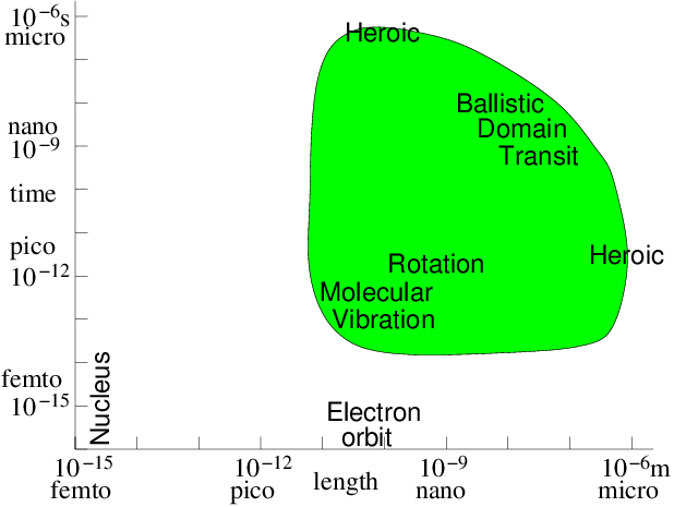
modelling time-scale. Fig.&nbsp;<a href="chap10.xml#timespacescalel">10.1</a> illustrates the
computationally feasible space and time-scale region (shaded) indicating the
approximate location of a few key phenomena.
<div class="p"><!----></div>

<div class="p"><!----></div>
<a id="tth_fIg10.1">
</a>   <img src="figures/timespacescale.png" alt="figures/timespacescale.png" /><a id="timespacescale">
</a>
  
<div style="text-align:center">Figure 10.1: Approximate space and time scales for Molecular Dynamics
    atomistic simulation of condensed matter. Molecular vibration must
    be accommodated. Then computations of heroic effort are required
    to explore many orders of magnitude above
    it.<a id="timespacescalel">
</a></div>

<div class="p"><!----></div>
For materials modelling where we are considering atoms whose thermal
velocities are perhaps <math xmlns="http://www.w3.org/1998/Math/MathML">
<mrow><mn>1000</mn></mrow></math>m/s, moving over lengths perhaps
<math xmlns="http://www.w3.org/1998/Math/MathML">
<mrow>
<msup><mrow><mn>10</mn></mrow><mrow><mo>-</mo><mn>7</mn></mrow>
</msup>
</mrow></math>m, the required rough time duration is <math xmlns="http://www.w3.org/1998/Math/MathML">
<mrow>
<msup><mrow><mn>10</mn></mrow><mrow><mo>-</mo><mn>10</mn></mrow>
</msup>
</mrow></math>s for
<em>molecular transit</em><a 
id="molecular_speed101576"></a>. This is far longer
than the characteristic time of motion of electrons within the atoms
themselves, which is approximately the atomic size <math xmlns="http://www.w3.org/1998/Math/MathML">
<mrow>
<msup><mrow><mn>10</mn></mrow><mrow><mo>-</mo><mn>10</mn></mrow>
</msup>
</mrow></math>m divided
by the electron velocity at say 10eV energy <math xmlns="http://www.w3.org/1998/Math/MathML">
<mrow>
<msup><mrow><mn>10</mn></mrow><mrow><mn>6</mn></mrow>
</msup>
</mrow></math>m/s: a time of
<math xmlns="http://www.w3.org/1998/Math/MathML">
<mrow>
<msup><mrow><mn>10</mn></mrow><mrow><mo>-</mo><mn>16</mn></mrow>
</msup>
</mrow></math>s for <em>electronic configuration</em>. This 1 million factor
time range is too great to span routinely. So atomistic modelling
usually needs to represent the atomic physics of the electron
configurations in molecules in some averaged approximate way. This
representation can sometimes be calculated on the basis of numerical
solution of quantum mechanics<a 
id="quantum_mechanics101577"></a>, but we won't
address that aspect of the problem. On the other hand, the motions of
the atomic nuclei arising from <em>molecular
  vibrations</em><a 
id="molecular_vibration101578"></a> has typical
timescale <math xmlns="http://www.w3.org/1998/Math/MathML">
<mrow><mo>~</mo>
<msup><mrow><mn>10</mn></mrow><mrow><mo>-</mo><mn>13</mn></mrow>
</msup>
</mrow></math>s: at least 1000 times longer than
electrons. This is managable, and indeed <em>must</em> be resolved, if
the dynamics of a lattice<a 
id="lattice_crystal101579"></a> are to be modelled.

<div class="p"><!----></div>
<a id="tth_fIg10.2">
</a>   <img src="figures/FCC30x30x30grey3.jpg" alt="figures/FCC30x30x30grey3.jpg" /><a id="FCC30x30x30grey3">
</a>
  
<div style="text-align:center">Figure 10.2: Example of a crystal lattice atomistic simulation in three
    dimensions. Study of a region of nanocrystaline metal with 840,000
    atoms ready to be deformed. (Courtesy: Ju Li, Massachusetts
    Institute of Technology.)<a id="VICfig">
</a></div>

<div class="p"><!----></div>
Atomistic modelling therefore represents the interatomic forces
arising<a 
id="force_interatomic101580"></a><a 
id="interatomic_force101581"></a> from
electron orbital interactions <em>only approximately</em>, as time
averages over electronic orbits or oscillations. But it follows the
atoms themselves in their motions in response to the interatomic
forces.  The atoms are represented as classical particles interacting
via a force field. This approach is sometimes called Molecular
Dynamics<a 
id="molecular_dynamics101582"></a>. It dates from as early as
1956<a href="footnote.xml#tthFtNtAGB" id="tthFrefAGB"><math xmlns="http://www.w3.org/1998/Math/MathML">
<mrow>
<msup><mrow></mrow><mrow><mn>61</mn></mrow>
</msup>
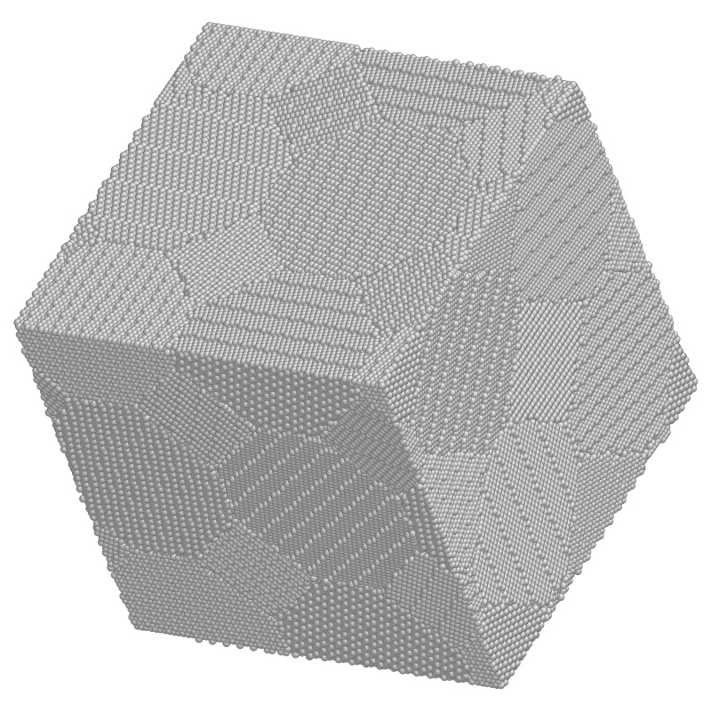
</mrow></math></a>. A modern example is shown in Fig.&nbsp;<a href="chap10.xml#VICfig">10.2</a>.

<div class="p"><!----></div>
The way a simulation works then is in outline

<div class="p"><!----></div>
<div class="small">
<table>
<tr><td align="left">1. </td><td align="left">Calculate the force at current position <math xmlns="http://www.w3.org/1998/Math/MathML">
<mrow><mi mathvariant="bold-italic">x</mi></mrow></math> on each particle
  due to all the others.</td></tr>
<tr><td align="left">2. </td><td align="left">Accelerate and move particles for <math xmlns="http://www.w3.org/1998/Math/MathML">
<mrow><mi mathvariant="italic">&Delta;</mi><mi>t</mi></mrow></math>, getting
  new velocities <math xmlns="http://www.w3.org/1998/Math/MathML">
<mrow><mi mathvariant="bold-italic">v</mi></mrow></math> and positions <math xmlns="http://www.w3.org/1998/Math/MathML">
<mrow><mi mathvariant="bold-italic">x</mi></mrow></math>.</td></tr>
<tr><td align="left">3. </td><td align="left">Repeat from 1.
</td></tr></table>
</div>

<div class="p"><!----></div>
Generally a fast second order accurate scheme for the acceleration and
motion (stage 2) is needed. One frequently used is the leap-frog
scheme. Another is called the Verlet<a 
id="Verlet_scheme101583"></a> scheme,
which can be expressed as
<a id="Verlet">
</a><br />
<table width="100%"><tr><td align="center">
    <math xmlns="http://www.w3.org/1998/Math/MathML">
    <mstyle displaystyle="true"><mrow>
<mtable displaystyle="true" align="right" width="80%">
<mtr><mtd columnalign="right" columnspan="1"><mrow>
<msub><mrow><mi mathvariant="bold-italic">x</mi></mrow><mrow><mi>n</mi><mo>+</mo><mn>1</mn></mrow>
</msub>
</mrow>
</mtd><mtd columnalign="left">
<mrow><mo>=</mo></mrow>
</mtd><mtd columnalign="left">
<mrow>
<msub><mrow><mi mathvariant="bold-italic">x</mi></mrow><mrow><mi>n</mi></mrow>
</msub>
<mo>+</mo>
<msub><mrow><mi mathvariant="bold-italic">v</mi></mrow><mrow><mi>n</mi></mrow>
</msub>
<mi mathvariant="italic">&Delta;</mi><mi>t</mi><mo>+</mo>
<msub><mrow><mi mathvariant="bold-italic">a</mi></mrow><mrow><mi>n</mi></mrow>
</msub>
<mi mathvariant="italic">&Delta;</mi>
<msup><mrow><mi>t</mi></mrow><mrow><mn>2</mn></mrow>
</msup>
<mo stretchy="false">/</mo><mn>2</mn></mrow>
</mtd></mtr>
<mtr><mtd columnalign="right" columnspan="1"><mrow>
<msub><mrow><mi mathvariant="bold-italic">v</mi></mrow><mrow><mi>n</mi><mo>+</mo><mn>1</mn></mrow>
</msub>
</mrow>
</mtd><mtd columnalign="left">
<mrow><mo>=</mo></mrow>
</mtd><mtd columnalign="left">
<mrow>
<msub><mrow><mi mathvariant="bold-italic">v</mi></mrow><mrow><mi>n</mi></mrow>
</msub>
<mo>+</mo><mo stretchy="false">(</mo>
<msub><mrow><mi mathvariant="bold-italic">a</mi></mrow><mrow><mi>n</mi></mrow>
</msub>
<mo>+</mo>
<msub><mrow><mi mathvariant="bold-italic">a</mi></mrow><mrow><mi>n</mi><mo>+</mo><mn>1</mn></mrow>
</msub>
<mo stretchy="false">)</mo><mi mathvariant="italic">&Delta;</mi><mi>t</mi><mo stretchy="false">/</mo><mn>2</mn></mrow>
</mtd><mtd columnalign="right">&emsp;&emsp;&emsp;&emsp;&emsp;&emsp;<mo stretchy="false">(</mo><mn>10</mn><mo>.</mo><mn>1</mn><mo stretchy="false">)</mo></mtd></mtr>
</mtable>
</mrow>
    </mstyle></math>
</td></tr></table>
<br />

where <math xmlns="http://www.w3.org/1998/Math/MathML">
<mrow>
<msub><mrow><mi mathvariant="bold-italic">a</mi></mrow><mrow><mi>n</mi></mrow>
</msub>
</mrow></math> is the acceleration corresponding to position
<math xmlns="http://www.w3.org/1998/Math/MathML">
<mrow>
<msub><mrow><mi mathvariant="bold-italic">x</mi></mrow><mrow><mi>n</mi></mrow>
</msub>
</mrow></math>.<a href="footnote.xml#tthFtNtAGC" id="tthFrefAGC"><math xmlns="http://www.w3.org/1998/Math/MathML">
<mrow>
<msup><mrow></mrow><mrow><mn>62</mn></mrow>
</msup>
</mrow></math></a>

<div class="p"><!----></div>
We also usually need to store a record of where the particles go,
since that is the major result of our simulation. And we need methods
to analyse and visualize the large amount of data that will result: the
number of steps <math xmlns="http://www.w3.org/1998/Math/MathML">
<mrow>
<msub><mrow><mi>N</mi></mrow><mrow><mi>t</mi></mrow>
</msub>
</mrow></math> times the number of particles <math xmlns="http://www.w3.org/1998/Math/MathML">
<mrow>
<msub><mrow><mi>N</mi></mrow><mrow><mi>p</mi></mrow>
</msub>
</mrow></math> times at
least 6 (3 space, and 3 velocity) components.

<div class="p"><!----></div>
     <a id="tth_sEc10.1.1"></a><h3>
10.1.1&nbsp;&nbsp;Atomic/Molecular Forces and Potentials</h3>

<div class="p"><!----></div>
The simplest type of forces, but still useful for a wide range of
physical situations, are particle-pair attraction and repulsion. Such
forces act along the vector <math xmlns="http://www.w3.org/1998/Math/MathML">
<mrow><mi mathvariant="bold-italic">r</mi><mo>=</mo>
<msub><mrow><mi mathvariant="bold-italic">x</mi></mrow><mrow><mn>1</mn></mrow>
</msub>
<mo>-</mo>
<msub><mrow><mi mathvariant="bold-italic">x</mi></mrow><mrow><mn>2</mn></mrow>
</msub>
</mrow></math> between the
particle positions, and have a magnitude that depends only upon the
distance <math xmlns="http://www.w3.org/1998/Math/MathML">
<mrow><mi>r</mi><mo>=</mo><mo stretchy="false">&verbar;</mo>
<msub><mrow><mi mathvariant="bold-italic">x</mi></mrow><mrow><mn>1</mn></mrow>
</msub>
<mo>-</mo>
<msub><mrow><mi mathvariant="bold-italic">x</mi></mrow><mrow><mn>2</mn></mrow>
</msub>
<mo stretchy="false">&verbar;</mo></mrow></math> between them. An example might be
the inverse-square electric force between two charges <math xmlns="http://www.w3.org/1998/Math/MathML">
<mrow>
<msub><mrow><mi>q</mi></mrow><mrow><mn>1</mn></mrow>
</msub>
</mrow></math> and <math xmlns="http://www.w3.org/1998/Math/MathML">
<mrow>
<msub><mrow><mi>q</mi></mrow><mrow><mn>2</mn></mrow>
</msub>
</mrow></math>,
<math xmlns="http://www.w3.org/1998/Math/MathML">
<mrow><mi mathvariant="bold-italic">F</mi><mo>=</mo><mo stretchy="false">(</mo>
<msub><mrow><mi>q</mi></mrow><mrow><mn>1</mn></mrow>
</msub>

<msub><mrow><mi>q</mi></mrow><mrow><mn>2</mn></mrow>
</msub>
<mo stretchy="false">/</mo><mn>4</mn><mi mathvariant="italic">&pi;</mi>
<msub><mrow><mi mathvariant="italic">&epsi;</mi></mrow><mrow><mn>0</mn></mrow>
</msub>
<mo stretchy="false">)</mo><mi mathvariant="bold-italic">r</mi><mo stretchy="false">/</mo>
<msup><mrow><mi>r</mi></mrow><mrow><mn>3</mn></mrow>
</msup>
</mrow></math>. But for atomistic
simulation more usually neutral particles are being modelled whose
force changes from mutual attraction at longer distances to mutual
repulsion at short distances. 
<div class="p"><!----></div>
<a id="tth_fIg10.3">
</a>   <img src="figures/lennardjones.png" alt="figures/lennardjones.png" /><a id="lennardjones">
</a>
  (a) &nbsp;&nbsp;&nbsp;&nbsp;&nbsp;&nbsp;&nbsp;&nbsp;&nbsp;&nbsp;&nbsp;&nbsp;&nbsp;&nbsp;&nbsp;&nbsp;&nbsp;&nbsp;&nbsp;&nbsp;&nbsp;&nbsp;&nbsp;&nbsp;&nbsp;&nbsp;&nbsp;&nbsp;&nbsp;&nbsp;&nbsp;&nbsp;&nbsp;&nbsp;&nbsp;&nbsp;&nbsp;&nbsp;
  <img src="figures/morse.png" alt="figures/morse.png" /><a id="morse">
</a>(b) &nbsp;&nbsp;&nbsp;&nbsp;&nbsp;&nbsp;&nbsp;&nbsp;&nbsp;&nbsp;&nbsp;&nbsp;&nbsp;&nbsp;&nbsp;&nbsp;&nbsp;&nbsp;&nbsp;&nbsp;&nbsp;&nbsp;&nbsp;&nbsp;&nbsp;&nbsp;&nbsp;&nbsp;&nbsp;&nbsp;&nbsp;&nbsp;&nbsp;&nbsp;&nbsp;&nbsp;&nbsp;
  
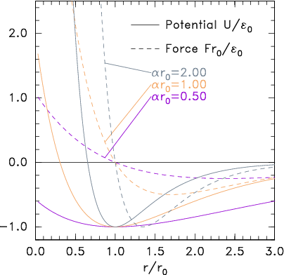
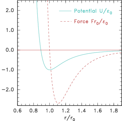
<div style="text-align:center">Figure 10.3: Potential and corresponding force forms for (a)
    Lennard-Jones (eq.&nbsp;<a href="chap10.xml#lennard-jones">10.2</a>) and (b) Morse (eq.&nbsp;    <a href="chap10.xml#Morse">10.3</a>) expressions.<a id="forceforms">
</a></div>
  

<div class="p"><!----></div>
A very common form of interatomic<a 
id="interatomic_potential101584"></a>
potential that gives this kind of attraction and repulsion is the
Lennard-Jones<a 
id="Lennard-Jones_potential101585"></a> (12:6) potential (see
Fig.&nbsp;<a href="chap10.xml#forceforms">10.3</a>(a))
<a id="lennard-jones">
</a><br />
<table width="100%"><tr><td align="center">
    <math xmlns="http://www.w3.org/1998/Math/MathML">
    <mstyle displaystyle="true"><mrow><mi mathvariant="bold-italic">F</mi><mo>=</mo><mo>-</mo><mo>&nabla;</mo><mi>U</mi><mi>&emsp;&emsp;&emsp;&emsp;&emsp;&emsp;</mi>
<mtext>with</mtext>
<mi>&emsp;&emsp;&emsp;&emsp;&emsp;&emsp;</mi><mi>U</mi><mo>=</mo>
<msub><mrow><mstyle fontfamily="helvetica"><mi fontstyle="italic">E</mi></mstyle></mrow>
<mrow><mn>0</mn></mrow>
</msub>
<mrow><mo>[</mo>
<msup><mrow><mo>(</mo>
<mfrac><mrow>
<msub><mrow><mi>r</mi></mrow><mrow><mn>0</mn></mrow>
</msub>
</mrow>
<mrow><mi>r</mi></mrow>
</mfrac>
<mo>)</mo></mrow><mrow><mn>12</mn></mrow>
</msup>
<mo>-</mo><mn>2</mn>
<msup><mrow><mo>(</mo>
<mfrac><mrow>
<msub><mrow><mi>r</mi></mrow><mrow><mn>0</mn></mrow>
</msub>
</mrow>
<mrow><mi>r</mi></mrow>
</mfrac>
<mo>)</mo></mrow><mrow><mn>6</mn></mrow>
</msup>
<mo>]</mo></mrow></mrow>
    </mstyle></math></td><td width="1">
    <math xmlns="http://www.w3.org/1998/Math/MathML">
    <mstyle displaystyle="true"><mrow><mo stretchy="false">(</mo><mn>10</mn><mo>.</mo><mn>2</mn><mo stretchy="false">)</mo></mrow>
    </mstyle></math>
</td></tr></table>


A simplicity, but also a weakness, in the Lennard-Jones form is that
it depends upon just two parameters, the typical energy <math xmlns="http://www.w3.org/1998/Math/MathML">
<mrow>
<msub><mrow><mstyle fontfamily="helvetica"><mi fontstyle="italic">E</mi></mstyle></mrow>
<mrow><mn>0</mn></mrow>
</msub>
</mrow></math>,
and the typical distance <math xmlns="http://www.w3.org/1998/Math/MathML">
<mrow>
<msub><mrow><mi>r</mi></mrow><mrow><mn>0</mn></mrow>
</msub>
</mrow></math>. The equilibrium distance,
corresponding to where the force (<math xmlns="http://www.w3.org/1998/Math/MathML">
<mrow><mo>-</mo><mi mathvariant="italic">dU</mi><mo stretchy="false">/</mo><mi mathvariant="italic">dr</mi></mrow></math>) is zero is, is <math xmlns="http://www.w3.org/1998/Math/MathML">
<mrow>
<msub><mrow><mi>r</mi></mrow><mrow><mn>0</mn></mrow>
</msub>
</mrow></math>. At
this spacing the binding energy is <math xmlns="http://www.w3.org/1998/Math/MathML">
<mrow>
<msub><mrow><mstyle fontfamily="helvetica"><mi fontstyle="italic">E</mi></mstyle></mrow>
<mrow><mn>0</mn></mrow>
</msub>
</mrow></math>. The maximum
attractive force occurs where <math xmlns="http://www.w3.org/1998/Math/MathML">
<mrow>
<msup><mrow><mi>d</mi></mrow><mrow><mn>2</mn></mrow>
</msup>
<mi>U</mi><mo stretchy="false">/</mo>
<msup><mrow><mi mathvariant="italic">dr</mi></mrow><mrow><mn>2</mn></mrow>
</msup>
<mo>=</mo><mn>0</mn></mrow></math>, which is <math xmlns="http://www.w3.org/1998/Math/MathML">
<mrow><mi>r</mi><mo>=</mo><mn>1</mn><mo>.</mo><mn>109</mn>
<msub><mrow><mi>r</mi></mrow><mrow><mn>0</mn></mrow>
</msub>
</mrow></math>
and it has magnitude <math xmlns="http://www.w3.org/1998/Math/MathML">
<mrow><mn>2</mn><mo>.</mo><mn>69</mn>
<msub><mrow><mstyle fontfamily="helvetica"><mi fontstyle="italic">E</mi></mstyle></mrow>
<mrow><mn>0</mn></mrow>
</msub>
<mo stretchy="false">/</mo>
<msub><mrow><mi>r</mi></mrow><mrow><mn>0</mn></mrow>
</msub>
</mrow></math>. The weakness of having only
two parameters is that the spring-constant for the force, <math xmlns="http://www.w3.org/1998/Math/MathML">
<mrow>
<msup><mrow><mi>d</mi></mrow><mrow><mn>2</mn></mrow>
</msup>
<mi>U</mi><mo stretchy="false">/</mo>
<msup><mrow><mi mathvariant="italic">dr</mi></mrow><mrow><mn>2</mn></mrow>
</msup>
</mrow></math>,
near the the equilibrium position cannot be set independent of the
binding energy. An alternative force expression that allows this
independence, by having three parameters, is the 
Morse<a 
id="Morse_potential101586"></a> form
<a id="Morse">
</a><br />
<table width="100%"><tr><td align="center">
    <math xmlns="http://www.w3.org/1998/Math/MathML">
    <mstyle displaystyle="true"><mrow><mi>U</mi><mo>=</mo>
<msub><mrow><mstyle fontfamily="helvetica"><mi fontstyle="italic">E</mi></mstyle></mrow>
<mrow><mn>0</mn></mrow>
</msub>
<mrow><mo>(</mo>
<msup><mrow><mi fontstyle="normal">e</mi></mrow><mrow><mo>-</mo><mn>2</mn><mi mathvariant="italic">&alpha;</mi><mo stretchy="false">(</mo><mi>r</mi><mo>-</mo>
<msub><mrow><mi>r</mi></mrow><mrow><mn>0</mn></mrow>
</msub>
<mo stretchy="false">)</mo></mrow>
</msup>
<mo>-</mo><mn>2</mn>
<msup><mrow><mi fontstyle="normal">e</mi></mrow><mrow><mo>-</mo><mi mathvariant="italic">&alpha;</mi><mo stretchy="false">(</mo><mi>r</mi><mo>-</mo>
<msub><mrow><mi>r</mi></mrow><mrow><mn>0</mn></mrow>
</msub>
<mo stretchy="false">)</mo></mrow>
</msup>
<mo>)</mo></mrow><mo>.</mo></mrow>
    </mstyle></math></td><td width="1">
    <math xmlns="http://www.w3.org/1998/Math/MathML">
    <mstyle displaystyle="true"><mrow><mo stretchy="false">(</mo><mn>10</mn><mo>.</mo><mn>3</mn><mo stretchy="false">)</mo></mrow>
    </mstyle></math>
</td></tr></table>


Its force is zero at <math xmlns="http://www.w3.org/1998/Math/MathML">
<mrow>
<msub><mrow><mi>r</mi></mrow><mrow><mn>0</mn></mrow>
</msub>
</mrow></math>, where the binding energy is <math xmlns="http://www.w3.org/1998/Math/MathML">
<mrow>
<msub><mrow><mstyle fontfamily="helvetica"><mi fontstyle="italic">E</mi></mstyle></mrow>
<mrow><mn>0</mn></mrow>
</msub>
</mrow></math>;
but the spring constant there can be adjusted using the parameter
<math xmlns="http://www.w3.org/1998/Math/MathML">
<mrow><mi mathvariant="italic">&alpha;</mi></mrow></math>.
See Fig.&nbsp;<a href="chap10.xml#forceforms">10.3</a>(b).

<div class="p"><!----></div>
These simple two-particle, radial-force, forms omit several phenomena
that are important in molecular interactions in nature. These
additional phenomena include higher order potential interactions,
represented by the total potential energy of the entire assembly being given
as a heirarchy of sums of multiple-particle interactions
<a id="potlinter">
</a><br />
<table width="100%"><tr><td align="center">
    <math xmlns="http://www.w3.org/1998/Math/MathML">
    <mstyle displaystyle="true"><mrow><mi>U</mi><mo>=</mo>
<munder><mo>&sum;</mo><mrow><mi>i</mi></mrow>
</munder>

<msub><mrow><mi>U</mi></mrow><mrow><mn>1</mn></mrow>
</msub>
<mo stretchy="false">(</mo>
<msub><mrow><mi mathvariant="bold-italic">x</mi></mrow><mrow><mi>i</mi></mrow>
</msub>
<mo stretchy="false">)</mo><mo>+</mo>
<munder><mo>&sum;</mo><mrow><mi mathvariant="italic">ij</mi></mrow>
</munder>

<msub><mrow><mi>U</mi></mrow><mrow><mn>2</mn></mrow>
</msub>
<mo stretchy="false">(</mo>
<msub><mrow><mi mathvariant="bold-italic">x</mi></mrow><mrow><mi>i</mi></mrow>
</msub>
<mo>,</mo>
<msub><mrow><mi mathvariant="bold-italic">x</mi></mrow><mrow><mi>j</mi></mrow>
</msub>
<mo stretchy="false">)</mo><mo>+</mo>
<munder><mo>&sum;</mo><mrow><mi mathvariant="italic">ijk</mi></mrow>
</munder>

<msub><mrow><mi>U</mi></mrow><mrow><mn>3</mn></mrow>
</msub>
<mo stretchy="false">(</mo>
<msub><mrow><mi mathvariant="bold-italic">x</mi></mrow><mrow><mi>i</mi></mrow>
</msub>
<mo>,</mo>
<msub><mrow><mi mathvariant="bold-italic">x</mi></mrow><mrow><mi>j</mi></mrow>
</msub>
<mo>,</mo>
<msub><mrow><mi mathvariant="bold-italic">x</mi></mrow><mrow><mi>k</mi></mrow>
</msub>
<mo stretchy="false">)</mo><mo>+</mo><mo>&#x2026;</mo></mrow>
    </mstyle></math></td><td width="1">
    <math xmlns="http://www.w3.org/1998/Math/MathML">
    <mstyle displaystyle="true"><mrow><mo stretchy="false">(</mo><mn>10</mn><mo>.</mo><mn>4</mn><mo stretchy="false">)</mo></mrow>
    </mstyle></math>
</td></tr></table>


where the subscripts <math xmlns="http://www.w3.org/1998/Math/MathML">
<mrow><mi>i</mi><mo>,</mo><mi>j</mi><mo>,</mo><mo>&#x2026;</mo></mrow></math> refer to different particles.
The force on a particular particle <math xmlns="http://www.w3.org/1998/Math/MathML">
<mrow><mi>l</mi></mrow></math> is then
<math xmlns="http://www.w3.org/1998/Math/MathML">
<mrow><mo>-</mo>
<mfrac><mrow><mo>&part;</mo></mrow>
<mrow><mo>&part;</mo>
<msub><mrow><mi mathvariant="bold-italic">x</mi></mrow><mrow><mi>l</mi></mrow>
</msub>
</mrow>
</mfrac>
<mi>U</mi></mrow></math>.  The first term <math xmlns="http://www.w3.org/1998/Math/MathML">
<mrow>
<msub><mrow><mi>U</mi></mrow><mrow><mn>1</mn></mrow>
</msub>
</mrow></math> represents a
background force field. The second represents the pairwise force that
we've so far been discussing. We've been considering the particular
case where <math xmlns="http://www.w3.org/1998/Math/MathML">
<mrow>
<msub><mrow><mi>U</mi></mrow><mrow><mn>2</mn></mrow>
</msub>
</mrow></math> depends only on <math xmlns="http://www.w3.org/1998/Math/MathML">
<mrow><mi>r</mi><mo>=</mo><mo stretchy="false">&verbar;</mo>
<msub><mrow><mi mathvariant="bold-italic">x</mi></mrow><mrow><mi>i</mi></mrow>
</msub>
<mo>-</mo>
<msub><mrow><mi mathvariant="bold-italic">x</mi></mrow><mrow><mi>j</mi></mrow>
</msub>
<mo stretchy="false">&verbar;</mo></mrow></math>. The third
(and higher) terms represent possible multi-particle correlation
forces. They are often called "cluster" potential
terms<a 
id="cluster_potential101587"></a>. 

<div class="p"><!----></div>
Other force laws between multi-atom molecules might include the
orientation of the molecule bonds. In that case, internal orientation
parameters would have to be introduced or else the molecule's
individual atoms themselves represented by particles whose bonds are
modelled using force laws appropriate to them. They could be
represented as a third or probably at least fourth order series for
the potential.

<div class="p"><!----></div>
     <a id="tth_sEc10.1.2"></a><h3>
10.1.2&nbsp;&nbsp;Computational requirements</h3>

<div class="p"><!----></div>
If there are <math xmlns="http://www.w3.org/1998/Math/MathML">
<mrow>
<msub><mrow><mi>N</mi></mrow><mrow><mi>p</mi></mrow>
</msub>
</mrow></math> particles, then to evaluate<a 
id="force_evaluation101588"></a>
the force on particle <math xmlns="http://www.w3.org/1998/Math/MathML">
<mrow><mi>i</mi></mrow></math> from all the other particles <math xmlns="http://www.w3.org/1998/Math/MathML">
<mrow><mi>j</mi></mrow></math>, requires
<math xmlns="http://www.w3.org/1998/Math/MathML">
<mrow>
<msub><mrow><mi>N</mi></mrow><mrow><mi>p</mi></mrow>
</msub>
</mrow></math> force evaluations for pair-forces (<math xmlns="http://www.w3.org/1998/Math/MathML">
<mrow>
<msub><mrow><mi>U</mi></mrow><mrow><mn>2</mn></mrow>
</msub>
</mrow></math> term). It requires
<math xmlns="http://www.w3.org/1998/Math/MathML">
<mrow>
<msubsup><mrow><mi>N</mi></mrow><mrow><mi>p</mi> </mrow>
<mrow><mn>2</mn></mrow></msubsup>
</mrow></math> for three-particle (<math xmlns="http://www.w3.org/1998/Math/MathML">
<mrow>
<msub><mrow><mi>U</mi></mrow><mrow><mn>3</mn></mrow>
</msub>
</mrow></math>) terms and so on. The force
calculation needs to be done for all the particles at each step, so if
we include even just the pair-forces for all particles, <math xmlns="http://www.w3.org/1998/Math/MathML">
<mrow>
<msubsup><mrow><mi>N</mi></mrow><mrow><mi>p</mi> </mrow>
<mrow><mn>2</mn></mrow></msubsup>
</mrow></math> force
terms must be evaluated. This is too much. For example, a million
particles would require <math xmlns="http://www.w3.org/1998/Math/MathML">
<mrow>
<msup><mrow><mn>10</mn></mrow><mrow><mn>12</mn></mrow>
</msup>
</mrow></math> pair force evaluations per time
step. Computational resources would be 
overwhelmed<a 
id="cost__computational__pair_force101589"></a>.  
Therefore the most important enabling
simplification of a practical atomistic simulation is to reduce the
number of force evaluations till it is not much worse than linear in
<math xmlns="http://www.w3.org/1998/Math/MathML">
<mrow>
<msub><mrow><mi>N</mi></mrow><mrow><mi>p</mi></mrow>
</msub>
</mrow></math>. This can be done by taking advantage of the fact that the force
laws between neutral atoms have a rather 
short range<a 
id="range_of_force101590"></a>; 
so the forces can be ignored for particle spacings greater
than some modest length. In reality we only need to calculate the
force contributions from a moderately small number of nearby particles
on each particle <math xmlns="http://www.w3.org/1998/Math/MathML">
<mrow><mi>i</mi></mrow></math>. It is not sufficient to look at the position of
all the other particles at each step and decide whether they are near
enough to worry about. That decision is itself an order <math xmlns="http://www.w3.org/1998/Math/MathML">
<mrow>
<msub><mrow><mi>N</mi></mrow><mrow><mi>p</mi></mrow>
</msub>
</mrow></math> cost per
particle (<math xmlns="http://www.w3.org/1998/Math/MathML">
<mrow>
<msubsup><mrow><mi>N</mi></mrow><mrow><mi>p</mi> </mrow>
<mrow><mn>2</mn></mrow></msubsup>
</mrow></math> total). Even if it's a bit cheaper than actually
evaluating the force, it won't do. Instead we have to keep track, in
some possibly approximate way, of which of the other particles are
close enough to the particle <math xmlns="http://www.w3.org/1998/Math/MathML">
<mrow><mi>i</mi></mrow></math> to matter to it.

<div class="p"><!----></div>
There are broadly two ways of doing this. Either we literally keep a
list of near neighbors<a 
id="neighbor101591"></a> associated with each
particle. Or else we divide up the volume under consideration into
much smaller blocks and adopt the policy of only examining the
particles in its own block and the neighboring
blocks<a 
id="block_spatial101592"></a>.  Either of these will obviously work for
a crystal lattice<a 
id="lattice_crystal101593"></a><a 
id="crystal_lattice101594"></a> type
problem, modelling a solid, because the atoms hardly ever change their
nearest neighbors, or the members of blocks.  But in liquids or gases
the particles can move sufficiently that their neighbors or blocks are
changing. To recalculate which particles are neighbors costs <math xmlns="http://www.w3.org/1998/Math/MathML">
<mrow><mo>~</mo>
<msubsup><mrow><mi>N</mi></mrow><mrow><mi>p</mi> </mrow>
<mrow><mn>2</mn></mrow></msubsup>
</mrow></math>. However, there are ways to avoid having to do the neighbor
determination every step. If we do it rarely enough, we reduce the
cost scaling.

<div class="p"><!----></div>

<b>Neighbor List Algorithm&nbsp;&nbsp;</b><a 
id="neighbor_list101595"></a>
 A common way to maintain an
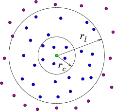
adequately accurate neighbor list is as follows. See Fig.&nbsp;<a href="chap10.xml#lneighborlist">10.4</a>.

<div class="p"><!----></div>
<a id="tth_fIg10.4">
</a>   <img src="figures/neigbors.png" alt="figures/neigbors.png" /><a id="neigbors">
</a>
  (a)&nbsp;&nbsp;&nbsp;&nbsp;&nbsp;&nbsp;&nbsp;&nbsp;&nbsp;&nbsp;&nbsp;&nbsp;&nbsp;&nbsp;&nbsp;&nbsp;&nbsp;&nbsp;&nbsp;&nbsp;&nbsp;&nbsp;&nbsp;&nbsp;&nbsp;&nbsp;&nbsp;&nbsp;&nbsp;&nbsp;&nbsp;&nbsp; 
  <img src="figures/blocks.png" alt="figures/blocks.png" /><a id="blocks">
</a>(b)&nbsp;&nbsp;&nbsp;&nbsp;&nbsp;&nbsp;&nbsp;&nbsp;&nbsp;&nbsp;&nbsp;&nbsp;&nbsp;&nbsp;&nbsp;&nbsp;&nbsp;&nbsp;&nbsp;&nbsp;&nbsp;&nbsp;&nbsp;&nbsp;&nbsp;&nbsp;&nbsp;&nbsp;&nbsp;&nbsp;&nbsp;
  
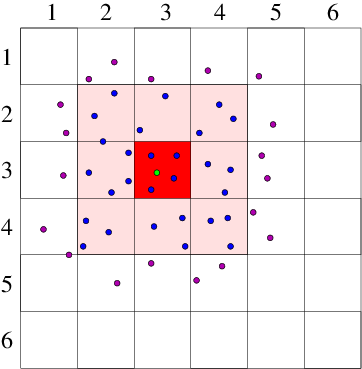
<div style="text-align:center">Figure 10.4: Neighbor List (a), and Block (b), algorithms enable testing
    only nearby particles for force influence. The neigbors whose
    influence must be calculated are inside the radius <math xmlns="http://www.w3.org/1998/Math/MathML">
<mrow>
<msub><mrow><mi>r</mi></mrow><mrow><mi>l</mi></mrow>
</msub>
</mrow></math> or inside
    the shaded region.<a id="lneighborlist">
</a></div>

<div class="p"><!----></div>
Suppose <math xmlns="http://www.w3.org/1998/Math/MathML">
<mrow>
<msub><mrow><mi>r</mi></mrow><mrow><mi>c</mi></mrow>
</msub>
</mrow></math> is the
cutoff radius beyond which interparticle forces are negligible. For
each particle <math xmlns="http://www.w3.org/1998/Math/MathML">
<mrow><mi>i</mi></mrow></math>, designate as neighbors particles within a larger
sphere <math xmlns="http://www.w3.org/1998/Math/MathML">
<mrow><mo stretchy="false">&verbar;</mo>
<msub><mrow><mi mathvariant="bold-italic">x</mi></mrow><mrow><mi>j</mi></mrow>
</msub>
<mo>-</mo>
<msub><mrow><mi mathvariant="bold-italic">x</mi></mrow><mrow><mi>i</mi></mrow>
</msub>
<mo stretchy="false">&verbar;</mo><mo>=</mo><mi>r</mi><mo>&lt;</mo>
<msub><mrow><mi>r</mi></mrow><mrow><mi>l</mi></mrow>
</msub>
</mrow></math>. Suppose the fastest speed a
particle has is <math xmlns="http://www.w3.org/1998/Math/MathML">
<mrow>
<msub><mrow><mi>v</mi></mrow><mrow><mi mathvariant="italic">max</mi></mrow>
</msub>
</mrow></math>; then we know that no particle, starting
from outside the sphere <math xmlns="http://www.w3.org/1998/Math/MathML">
<mrow>
<msub><mrow><mi>r</mi></mrow><mrow><mi>l</mi></mrow>
</msub>
</mrow></math>, can reach the sphere <math xmlns="http://www.w3.org/1998/Math/MathML">
<mrow>
<msub><mrow><mi>r</mi></mrow><mrow><mi>c</mi></mrow>
</msub>
</mrow></math> in less than
a time <math xmlns="http://www.w3.org/1998/Math/MathML">
<mrow><mo stretchy="false">(</mo>
<msub><mrow><mi>r</mi></mrow><mrow><mi>l</mi></mrow>
</msub>
<mo>-</mo>
<msub><mrow><mi>r</mi></mrow><mrow><mi>c</mi></mrow>
</msub>
<mo stretchy="false">)</mo><mo stretchy="false">/</mo>
<msub><mrow><mi>v</mi></mrow><mrow><mi mathvariant="italic">max</mi></mrow>
</msub>
</mrow></math>, that is, in fewer timesteps than
<math xmlns="http://www.w3.org/1998/Math/MathML">
<mrow>
<msub><mrow><mi>N</mi></mrow><mrow><mi>l</mi></mrow>
</msub>
<mo>=</mo><mo stretchy="false">(</mo>
<msub><mrow><mi>r</mi></mrow><mrow><mi>l</mi></mrow>
</msub>
<mo>-</mo>
<msub><mrow><mi>r</mi></mrow><mrow><mi>c</mi></mrow>
</msub>
<mo stretchy="false">)</mo><mo stretchy="false">/</mo>
<msub><mrow><mi>v</mi></mrow><mrow><mi mathvariant="italic">max</mi></mrow>
</msub>
<mi mathvariant="italic">&Delta;</mi><mi>t</mi></mrow></math>. Consequently, we need to update the
neighbor lists only every <math xmlns="http://www.w3.org/1998/Math/MathML">
<mrow>
<msub><mrow><mi>N</mi></mrow><mrow><mi>l</mi></mrow>
</msub>
</mrow></math> steps. The average neighbor list cost
per step is <math xmlns="http://www.w3.org/1998/Math/MathML">
<mrow>
<msubsup><mrow><mi>N</mi></mrow><mrow><mi>p</mi> </mrow>
<mrow><mn>2</mn></mrow></msubsup>
<mo stretchy="false">/</mo>
<msub><mrow><mi>N</mi></mrow><mrow><mi>l</mi></mrow>
</msub>
</mrow></math>. This is smaller than <math xmlns="http://www.w3.org/1998/Math/MathML">
<mrow>
<msubsup><mrow><mi>N</mi></mrow><mrow><mi>p</mi> </mrow>
<mrow><mn>2</mn></mrow></msubsup>
</mrow></math>, and if <math xmlns="http://www.w3.org/1998/Math/MathML">
<mrow>
<msub><mrow><mi>N</mi></mrow><mrow><mi>l</mi></mrow>
</msub>
</mrow></math> is large
(because the maximum velocity is small), much smaller. However, it is
still of order <math xmlns="http://www.w3.org/1998/Math/MathML">
<mrow>
<msubsup><mrow><mi>N</mi></mrow><mrow><mi>p</mi> </mrow>
<mrow><mn>2</mn></mrow></msubsup>
</mrow></math>.<a href="footnote.xml#tthFtNtAGD" id="tthFrefAGD"><math xmlns="http://www.w3.org/1998/Math/MathML">
<mrow>
<msup><mrow></mrow><mrow><mn>63</mn></mrow>
</msup>
</mrow></math></a>

<div class="p"><!----></div>

<b>Block Algorithm&nbsp;&nbsp;</b><a 
id="block_neigbor_algorithm101596"></a>
If the domain is divided into a large
number of blocks, each of which is bigger than the cutoff radius, then
we need to examine only particles that are in the same block or an
adjacent block. Adjacent blocks must be examined because a particle
near the boundary of a block might be influenced by particles just the
other side of that boundary. Suppose there are <math xmlns="http://www.w3.org/1998/Math/MathML">
<mrow>
<msub><mrow><mi>N</mi></mrow><mrow><mi>b</mi></mrow>
</msub>
</mrow></math> blocks. They
contain on average <math xmlns="http://www.w3.org/1998/Math/MathML">
<mrow>
<msub><mrow><mi>N</mi></mrow><mrow><mi>p</mi></mrow>
</msub>
<mo stretchy="false">/</mo>
<msub><mrow><mi>N</mi></mrow><mrow><mi>b</mi></mrow>
</msub>
</mrow></math> particles each. As the size of the
computational region increases, we can keep this ratio constant.  The
total number of neighboring particles we need to examine for each
particle <math xmlns="http://www.w3.org/1998/Math/MathML">
<mrow><mi>i</mi></mrow></math> is (in three dimensions) <math xmlns="http://www.w3.org/1998/Math/MathML">
<mrow>
<msup><mrow><mn>3</mn></mrow><mrow><mn>3</mn></mrow>
</msup>

<msub><mrow><mi>N</mi></mrow><mrow><mi>p</mi></mrow>
</msub>
<mo stretchy="false">/</mo>
<msub><mrow><mi>N</mi></mrow><mrow><mi>b</mi></mrow>
</msub>
<mo>&prop;</mo><mi mathvariant="italic">const</mi><mo>.</mo></mrow></math> Thus,
this block algorithm's step cost is <math xmlns="http://www.w3.org/1998/Math/MathML">
<mrow><mo>&prop;</mo>
<msub><mrow><mi>N</mi></mrow><mrow><mi>p</mi></mrow>
</msub>
</mrow></math>, linear in the
number of particles. But the constant of proportionality might be
quite large.  There is also an interesting question as to how the list
of particles in a block is maintained. One way to do this is to use a
linked list of pointers. However, such a linked list does not lend
itself readily to parallel data implementations, and there are
interesting forefront research questions as to the best practical way
of solving this problem.

<div class="p"><!----></div>
 <a id="tth_sEc10.2"></a><h2>
10.2&nbsp;&nbsp;Particle in Cell Codes</h2>

<div class="p"><!----></div>
<a 
id="particle-in-cell102597"></a> If the interparticle force law is of infinite
range, as it is, for example, with the
inverse-square<a 
id="inverse-square_interaction102598"></a> interactions of
charged particles in a plasma, or gravitating stars, then the
near-neighbor reduction of the force calculation does not work,
because there is no cutoff radius beyond which the interaction is
negligible. This problem is solved in a different way, by representing
the long-range interactions as the potential on a mesh of cells. This
approach is called "Particle in Cell" or PIC<a 
id="PIC102599"></a><a href="footnote.xml#tthFtNtAGE" id="tthFrefAGE"><math xmlns="http://www.w3.org/1998/Math/MathML">
<mrow>
<msup><mrow></mrow><mrow><mn>64</mn></mrow>
</msup>
</mrow></math></a>.

<div class="p"><!----></div>
Consider, for simplicity, a single species of charged particles (call
them electrons) of charge <math xmlns="http://www.w3.org/1998/Math/MathML">
<mrow><mi>q</mi></mrow></math> (<math xmlns="http://www.w3.org/1998/Math/MathML">
<mrow><mo>=</mo><mo>-</mo><mi>e</mi></mrow></math> for electrons<a 
id="electron102600"></a>, of
course), and mass <math xmlns="http://www.w3.org/1998/Math/MathML">
<mrow><mi>m</mi></mrow></math>. Positive ions<a 
id="ion102601"></a> could also be modelled
as particles, but for now take them to be represented by a smooth
neutralizing background of positive charge density <math xmlns="http://www.w3.org/1998/Math/MathML">
<mrow><mo>-</mo>
<msub><mrow><mi>n</mi></mrow><mrow><mi>i</mi></mrow>
</msub>
<mi>q</mi></mrow></math>. The
electrons move in a region of space divided into cells labelled with
index <math xmlns="http://www.w3.org/1998/Math/MathML">
<mrow><mi>j</mi></mrow></math> at positions <math xmlns="http://www.w3.org/1998/Math/MathML">
<mrow>
<msub><mrow><mi>x</mi></mrow><mrow><mi>j</mi></mrow>
</msub>
</mrow></math>. [Most modern PIC production codes are
multidimensional, but the explanations are easier in one dimension.]
They give rise to an electric potential <math xmlns="http://www.w3.org/1998/Math/MathML">
<mrow><mi mathvariant="italic">&phi;</mi></mrow></math>. Ignoring the
discreteness of the individual electrons, there is a smoothed-out
total (sum of electron and ion) charge density <math xmlns="http://www.w3.org/1998/Math/MathML">
<mrow>
<msub><mrow><mi mathvariant="italic">&rho;</mi></mrow><mrow><mi>q</mi></mrow>
</msub>
<mo stretchy="false">(</mo><mi>x</mi><mo stretchy="false">)</mo><mo>=</mo><mi>q</mi><mo stretchy="false">[</mo><mi>n</mi><mo stretchy="false">(</mo><mi>x</mi><mo stretchy="false">)</mo><mo>-</mo>
<msub><mrow><mi>n</mi></mrow><mrow><mi>i</mi></mrow>
</msub>
<mo stretchy="false">]</mo></mrow></math>.  The potential satisfies Poisson's
equation<a 
id="Poisson_equation102602"></a>
<a id="PICpoiss">
</a><br />
<table width="100%"><tr><td align="center">
    <math xmlns="http://www.w3.org/1998/Math/MathML">
    <mstyle displaystyle="true"><mrow>
<msup><mrow><mo>&nabla;</mo></mrow><mrow><mn>2</mn></mrow>
</msup>
<mi mathvariant="italic">&phi;</mi><mo>=</mo>
<mfrac><mrow>
<msup><mrow><mi>d</mi></mrow><mrow><mn>2</mn></mrow>
</msup>
<mi mathvariant="italic">&phi;</mi></mrow>
<mrow>
<msup><mrow><mi mathvariant="italic">dx</mi></mrow><mrow><mn>2</mn></mrow>
</msup>
</mrow>
</mfrac>
<mo>=</mo><mo>-</mo>
<mfrac><mrow>
<msub><mrow><mi mathvariant="italic">&rho;</mi></mrow><mrow><mi>q</mi></mrow>
</msub>
</mrow>
<mrow>
<msub><mrow><mi mathvariant="italic">&epsi;</mi></mrow><mrow><mn>0</mn></mrow>
</msub>
</mrow>
</mfrac>
<mo>=</mo><mo>-</mo>
<mfrac><mrow><mi>q</mi><mo stretchy="false">[</mo><mi>n</mi><mo stretchy="false">(</mo><mi>x</mi><mo stretchy="false">)</mo><mo>-</mo>
<msub><mrow><mi>n</mi></mrow><mrow><mi>i</mi></mrow>
</msub>
<mo stretchy="false">]</mo></mrow>
<mrow>
<msub><mrow><mi mathvariant="italic">&epsi;</mi></mrow><mrow><mn>0</mn></mrow>
</msub>
</mrow>
</mfrac>
</mrow>
    </mstyle></math></td><td width="1">
    <math xmlns="http://www.w3.org/1998/Math/MathML">
    <mstyle displaystyle="true"><mrow><mo stretchy="false">(</mo><mn>10</mn><mo>.</mo><mn>5</mn><mo stretchy="false">)</mo></mrow>
    </mstyle></math>
</td></tr></table>


We represent this potential discretely on the mesh: <math xmlns="http://www.w3.org/1998/Math/MathML">
<mrow>
<msub><mrow><mi mathvariant="italic">&phi;</mi></mrow><mrow><mi>i</mi></mrow>
</msub>
</mrow></math> and solve
it numerically using a standard elliptic solver.  The only new
feature is that we need to obtain a measure of smoothed-out density on
the mesh. We do this by assigning the charge density of the individual
electrons to the mesh in a systematic way. The simplest way to assign
it is to say 
that each electron's charge is assigned<a 
id="charge_assignment102603"></a> 
to the <em>Nearest Grid Point</em><a 
id="nearest_grid_point102604"></a> NGP. 
That's equivalent
to saying each electron is like a rod of length equal to the distance
<math xmlns="http://www.w3.org/1998/Math/MathML">
<mrow><mi mathvariant="italic">&Delta;</mi><mi>x</mi></mrow></math> between the grid points, and it contributes charge density
equal to <math xmlns="http://www.w3.org/1998/Math/MathML">
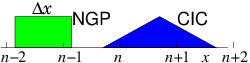
<mrow><mi>q</mi><mo stretchy="false">/</mo><mi mathvariant="italic">&Delta;</mi><mi>x</mi></mrow></math> from all positions along its length. See Fig.&nbsp;<a href="chap10.xml#chargeshapel">10.5</a>. The volume
of the cell is <math xmlns="http://www.w3.org/1998/Math/MathML">
<mrow><mi mathvariant="italic">&Delta;</mi><mi>x</mi></mrow></math> and the electron density is equal to the
number of particles whose charge is assigned to that cell divided by
the cell volume.

<div class="p"><!----></div>
<a id="tth_fIg10.5">
</a>   <img src="figures/chargeshape.png" alt="figures/chargeshape.png" /><a id="chargeshape">
</a>
  
<div style="text-align:center">Figure 10.5: Effective shapes for the NGP and CIC charge assignments.<a id="chargeshapel">
</a></div>

<div class="p"><!----></div>
Usually a continuous linear
interpolation is preferred, called the <em>Cloud In
  Cell</em><a 
id="cloud_in_cell102605"></a> CIC assignment. The
charge density assigned from each electron is equal to <math xmlns="http://www.w3.org/1998/Math/MathML">
<mrow><mi>q</mi><mo stretchy="false">/</mo><mi mathvariant="italic">&Delta;</mi><mi>x</mi></mrow></math> when
the electron is exactly at <math xmlns="http://www.w3.org/1998/Math/MathML">
<mrow>
<msub><mrow><mi>x</mi></mrow><mrow><mi>j</mi></mrow>
</msub>
</mrow></math>, and falls linearly, reaching zero when
the particle is at <math xmlns="http://www.w3.org/1998/Math/MathML">
<mrow>
<msub><mrow><mi>x</mi></mrow><mrow><mi>j</mi><mo>&PlusMinus;</mo><mn>1</mn></mrow>
</msub>
</mrow></math>. Thus the electron is like a rod of length
<math xmlns="http://www.w3.org/1998/Math/MathML">
<mrow><mn>2</mn><mi mathvariant="italic">&Delta;</mi><mi>x</mi></mrow></math> whose charge distribution is triangular. 

<div class="p"><!----></div>
The way the particle in cell code runs is this.

<div class="p"><!----></div>

<table>
<tr><td align="left">1.</td><td align="left">Assign the charge from all the particles onto the grid cells.</td></tr>
<tr><td align="left">2.</td><td align="left">Solve Poisson's equation to find the potential <math xmlns="http://www.w3.org/1998/Math/MathML">
<mrow>
<msub><mrow><mi mathvariant="italic">&phi;</mi></mrow><mrow><mi>j</mi></mrow>
</msub>
</mrow></math>.</td></tr>
<tr><td align="left">3.</td><td align="left">For each particle, find <math xmlns="http://www.w3.org/1998/Math/MathML">
<mrow><mo>&nabla;</mo><mi mathvariant="italic">&phi;</mi></mrow></math> at its position, <math xmlns="http://www.w3.org/1998/Math/MathML">
<mrow>
<msub><mrow><mi>x</mi></mrow><mrow><mi>i</mi></mrow>
</msub>
</mrow></math>, by
  interpolation from the <math xmlns="http://www.w3.org/1998/Math/MathML">
<mrow>
<msub><mrow><mi>x</mi></mrow><mrow><mi>j</mi></mrow>
</msub>
</mrow></math>.</td></tr>
<tr><td align="left">4.</td><td align="left">Accelerate, by the corresponding force, and move the particles.</td></tr>
<tr><td align="left">5.</td><td align="left">Repeat from 1.</td></tr></table>


<div class="p"><!----></div>
This process will simulate the behavior of the plasma accounting
realistically for the particle motion. So it is a kind of atomistic
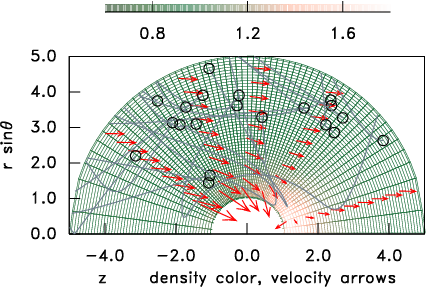
simulation. Fig.&nbsp;<a href="chap10.xml#scepticgrid">10.6</a> shows an illustration of an
example in a spherical computational domain.

<div class="p"><!----></div>
<a id="tth_fIg10.6">
</a>   <img src="figures/grid.png" alt="figures/grid.png" /><a id="grid">
</a>
  
<div style="text-align:center">Figure 10.6: A curved grid (relatively unusual for PIC) shaded to
    represent the density normalized to the distant value.
    A few representative particle orbits in the vicinity of a spherical
    object are shown, and arrows indicate the mean ion
    velocity.<a id="scepticgrid">
</a></div>

<div class="p"><!----></div>
Why introduce this cell mesh? Because this approach is computationally
far more efficient<a 
id="cost__computational__PIC102606"></a> than adding up the
inverse square law forces between individual particles. An atomistic
pair-force approach costs <math xmlns="http://www.w3.org/1998/Math/MathML">
<mrow><mo>~</mo>
<msubsup><mrow><mi>N</mi></mrow><mrow><mi>p</mi> </mrow>
<mrow><mn>2</mn></mrow></msubsup>
</mrow></math> per step. By contrast the
particle moving stage, once the force is known is <math xmlns="http://www.w3.org/1998/Math/MathML">
<mrow><mo>~</mo>
<msub><mrow><mi>N</mi></mrow><mrow><mi>p</mi></mrow>
</msub>
</mrow></math>. If the
potential grid has a total of <math xmlns="http://www.w3.org/1998/Math/MathML">
<mrow>
<msub><mrow><mi>N</mi></mrow><mrow><mi>g</mi></mrow>
</msub>
</mrow></math> points, then an efficient
iterative Poisson solution costs <math xmlns="http://www.w3.org/1998/Math/MathML">
<mrow><mo>~</mo>
<msub><mrow><mi>N</mi></mrow><mrow><mi>g</mi></mrow>
</msub>

<msubsup><mrow><mi>N</mi></mrow><mrow><mi>g</mi> </mrow>
<mrow><mn>1</mn><mo stretchy="false">/</mo>
<msub><mrow><mi>N</mi></mrow><mrow><mi>d</mi></mrow>
</msub>
</mrow></msubsup>
</mrow></math> per step, in
<math xmlns="http://www.w3.org/1998/Math/MathML">
<mrow>
<msub><mrow><mi>N</mi></mrow><mrow><mi>d</mi></mrow>
</msub>
</mrow></math> dimensions<a href="footnote.xml#tthFtNtAGF" id="tthFrefAGF"><math xmlns="http://www.w3.org/1998/Math/MathML">
<mrow>
<msup><mrow></mrow><mrow><mn>65</mn></mrow>
</msup>
</mrow></math></a>, or can
be done by tridiagonal elimination<a 
id="tridiagonal_elimination102607"></a> in
<math xmlns="http://www.w3.org/1998/Math/MathML">
<mrow><mo>~</mo>
<msub><mrow><mi>N</mi></mrow><mrow><mi>g</mi></mrow>
</msub>
</mrow></math> operations in one dimension. Generally the number of
particles per cell is fairly large, so <math xmlns="http://www.w3.org/1998/Math/MathML">
<mrow>
<msub><mrow><mi>N</mi></mrow><mrow><mi>g</mi></mrow>
</msub>
</mrow></math> is much smaller than
<math xmlns="http://www.w3.org/1998/Math/MathML">
<mrow>
<msub><mrow><mi>N</mi></mrow><mrow><mi>p</mi></mrow>
</msub>
</mrow></math> and the Poisson cost scales linearly or nearly linearly with
<math xmlns="http://www.w3.org/1998/Math/MathML">
<mrow>
<msub><mrow><mi>N</mi></mrow><mrow><mi>g</mi></mrow>
</msub>
</mrow></math>. Therefore for practical purposes, the costs are dominantly
those of interpolating the electric field to the particle and moving
it: an order <math xmlns="http://www.w3.org/1998/Math/MathML">
<mrow>
<msub><mrow><mi>N</mi></mrow><mrow><mi>p</mi></mrow>
</msub>
</mrow></math> cost, not <math xmlns="http://www.w3.org/1998/Math/MathML">
<mrow>
<msubsup><mrow><mi>N</mi></mrow><mrow><mi>p</mi> </mrow>
<mrow><mn>2</mn></mrow></msubsup>
</mrow></math> like the pair-force approach.

<div class="p"><!----></div>
Sometimes the dynamics of the ions is just as important to model as
the electrons. Then the ions must be treated through the PIC approach
as a second species of particles obeying Newton's law. Actually it is
sometimes advantageous to treat only the ions this way, and treat
electrons as a continuum whose density is a known function of
<math xmlns="http://www.w3.org/1998/Math/MathML">
<mrow><mi mathvariant="italic">&phi;</mi></mrow></math>. The latter approach is 
often called "Hybrid"<a 
id="hybrid_PIC102608"></a> PIC.

<div class="p"><!----></div>
<br /><br />     <a id="tth_sEc10.2.1"></a><h3>
10.2.1&nbsp;&nbsp;Boltzmann Equation Pseudoparticle Representation</h3>

<div class="p"><!----></div>
In a particle in cell code, the particles move and are tracked in
phase-space: <math xmlns="http://www.w3.org/1998/Math/MathML">
<mrow><mo stretchy="false">(</mo><mi mathvariant="bold-italic">x</mi><mo>,</mo><mi mathvariant="bold-italic">v</mi><mo stretchy="false">)</mo></mrow></math> is known at each time-step. A particle's
equation of motion in phase space is 
<a id="piccharac">
</a><br />
<table width="100%"><tr><td align="center">
    <math xmlns="http://www.w3.org/1998/Math/MathML">
    <mstyle displaystyle="true"><mrow>
<mfrac><mrow><mi>d</mi></mrow>
<mrow><mi mathvariant="italic">dt</mi></mrow>
</mfrac>
<mrow><mo>(</mo>
<mfrac linethickness="0"><mrow><mi mathvariant="bold-italic">x</mi></mrow>
<mrow><mi mathvariant="bold-italic">v</mi></mrow>
</mfrac>
<mo>)</mo></mrow><mo>=</mo><mrow><mo>(</mo>
<mfrac linethickness="0"><mrow><mi mathvariant="bold-italic">v</mi></mrow>
<mrow><mi mathvariant="bold-italic">a</mi></mrow>
</mfrac>
<mo>)</mo></mrow><mo>.</mo></mrow>
    </mstyle></math></td><td width="1">
    <math xmlns="http://www.w3.org/1998/Math/MathML">
    <mstyle displaystyle="true"><mrow><mo stretchy="false">(</mo><mn>10</mn><mo>.</mo><mn>6</mn><mo stretchy="false">)</mo></mrow>
    </mstyle></math>
</td></tr></table>


This is also the equation of motion of the <em>characteristics</em> of
the Boltzmann equation (<a href="chap8.xml#Boltzmann">8.12</a>,<a href="chap8.xml#orbitaccel">8.13</a>). Thus
advancing a PIC code with <math xmlns="http://www.w3.org/1998/Math/MathML">
<mrow>
<msub><mrow><mi>N</mi></mrow><mrow><mi>p</mi></mrow>
</msub>
</mrow></math> particles is equivalent to integrating
along <math xmlns="http://www.w3.org/1998/Math/MathML">
<mrow>
<msub><mrow><mi>N</mi></mrow><mrow><mi>p</mi></mrow>
</msub>
</mrow></math> characteristics of the Boltzmann equation. But what about
collisions<a 
id="collision_in_PIC_code102609"></a>?

<div class="p"><!----></div>
The remarkable thing about a PIC code, in its simplest implementation,
is that it has essentially <em>removed</em> all charged-particle
collisions. The grainy discreteness of the electrons, is smoothed away
by the process of assigning charge to the grid and then solving for
<math xmlns="http://www.w3.org/1998/Math/MathML">
<mrow><mi mathvariant="italic">&phi;</mi></mrow></math>. Therefore, unless we do something to put collisions back, the
PIC code actually represents integration along characteristics of the
<em>Vlasov</em> equation<a 
id="Vlasov_equation102610"></a>, the
<em>collisionless</em> Boltzmann equation. If we had instead used
(highly inefficiently) pair-forces, then the charged particle
collisions would have been retained.

<div class="p"><!----></div>
Because the collisions have been removed from the problem, the actual
magnitude of each particle's charge and mass no longer matters; only
the <em>ratio</em>, <math xmlns="http://www.w3.org/1998/Math/MathML">
<mrow><mi>q</mi><mo stretchy="false">/</mo><mi>m</mi></mrow></math>, appears in the acceleration, <math xmlns="http://www.w3.org/1998/Math/MathML">
<mrow><mi mathvariant="bold-italic">a</mi></mrow></math>, in
the Vlasov equation.  That means we can represent physical situations
that would in nature involve unmanagable numbers of physical electrons by
regarding the electrons (or ions) of our computation as
<em>pseudo-particles</em><a 
id="pseudo-particle102611"></a>. Each pseudo-particle corresponds to a very
large number of actual particles, reducing the number of computation
pseudo-particles to a managable total, and keeping the costs of the
computation within tolerable bounds. For our computation to remain a
faithful representation of the physical situation, we require only
that the resolution in phase-space, which depends upon the total
number of randomly distributed electrons, should be sufficient for whatever
phenomenon is being studied. We also require, of course, that the
potential mesh has sufficient spatial resolution.

<div class="p"><!----></div>
<a id="tth_fIg10.7">
</a>   <img src="figures/xes3.jpg" alt="figures/xes3.jpg" /><a id="xes3">
</a>
  
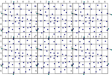
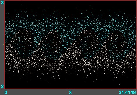
<div style="text-align:center">Figure 10.7: Example of phase-space locations of electrons. A
    one-dimensional <math xmlns="http://www.w3.org/1998/Math/MathML">
<mrow><mi>v</mi></mrow></math> versus <math xmlns="http://www.w3.org/1998/Math/MathML">
<mrow><mi>x</mi></mrow></math> calculation is illustrated, using
    the code XES1 (by Birdsall, Langdon, Verboncoeur and Vahedi,
    originally distributed with the text by Birdsall and Langdon) for
    two streams of particles giving rise to an instability whose
    wavelength is four times the domain length. Each electron position
    is marked as a point. Their motion can be viewed like a
    movie.<a id="xes3l">
</a></div>

<div class="p"><!----></div>
Particle in cell codes are a backbone of much computational plasma
physics, important for modelling semiconductor processing tools, space
interactions, accelerators, and fusion experiments. An example of a
one-dimensional PIC calculation is shown in Fig.&nbsp;<a href="chap10.xml#xes3l">10.7</a>. They are
particularly useful for collisionless or nearly collisionless problems
that are widespread in the field. They can also be modified to include
collisions of various different types, as the conditions require
them. In plasmas, though, charged-particle collisions are often
dominated by small scattering angles and are much better approximated
by a Fokker-Planck diffusion in phase space than by discrete events.

<div class="p"><!----></div>
     <a id="tth_sEc10.2.2"></a><h3>
10.2.2&nbsp;&nbsp;Direct Simulation Monte Carlo treatment of gas</h3>

<div class="p"><!----></div>
An approach that combines some of the features of PIC and atomistic
simulation, is the treatment of tenuous neutral gas behavior by what
have come to be called Direct Simulation Monte Carlo 
(DSMC)<a 
id="DSMC_codes102612"></a> codes.
These are for addressing situations where the ratio of the
mean-free-path<a 
id="mean-free-path102613"></a> of molecules to the 
characteristic spatial feature size
(the "Knudsen number")<a 
id="Knudsen_number102614"></a> is of order unity
(within a factor of 100 or so either way). Such situations occur in
very tenuous gases (e.g. orbital re-entry in space) or when the
features are microscopic. DSMC shares with PIC the features that the
domain is divided into a large number of cells, that 
pseudo-particles<a 
id="pseudo-particle102615"></a>
are used, and that collisions are represented in simplified way that
reduces computational cost and yet approximates physical
behavior. DMSC is also, in effect, integrating the Boltzmann equation
along characteristics, but in this case there's no acceleration term,
so the characteristics are straight lines.

<div class="p"><!----></div>
The pseudo-particles representing molecules are advanced in time, but
at each step, chosen somewhat shorter than a typical collision time,
they are examined to decide whether they have collided.  In order to
avoid a <math xmlns="http://www.w3.org/1998/Math/MathML">
<mrow>
<msubsup><mrow><mi>N</mi></mrow><mrow><mi>p</mi> </mrow>
<mrow><mn>2</mn></mrow></msubsup>
</mrow></math> cost, collisions are considered only with the
particles in the same cell of the grid. (This partitioning is all the
cells are used for.) The cells are chosen to have size smaller than a
mean-free-path, but not by much. They will generally have only a
modest number (perhaps 20-40) of pseudo-particles in each cell. The
number of individual molecules represented by each pseudo-particle is
adjusted to achieve this number per cell. 

<div class="p"><!----></div>
Whether a collision has occurred between two particles is decided
based only upon their relative <em>velocity</em>, not on their position
within the cell. This is the big approximation. A statistical test
using random numbers decides if and which collisions have happened.  A
collision changes the velocity of both colliding particles, in
accordance with the statistics of the collision cross-section and
corresponding kinematics. That way, momentum and energy are
appropriately conserved within the cell as a whole.  Steps are
iterated, and the overall behavior of the assembly of particles is
monitored and analysed to provide effective fluid parameters like
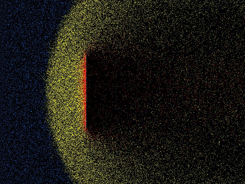
density, velocity, effective viscosity, and so on. Fig.&nbsp;<a href="chap10.xml#dsmcl">10.8</a>
shows an example from the code DSMC, v3.0 developed by Graeme Bird.
<div class="p"><!----></div>
<a id="tth_fIg10.8">
</a>   <img src="figures/dsmc.jpg" alt="figures/dsmc.jpg" /><a id="dsmc">
</a>
  
<div style="text-align:center">Figure 10.8: Example of position plot in two space dimensions of tenuous
    gas flow past a plate. Different colors (shadings) indicate molecules that
    have been influenced by the plate through collisions.<a id="dsmcl">
</a></div>

<div class="p"><!----></div>
     <a id="tth_sEc10.2.3"></a><h3>
10.2.3&nbsp;&nbsp;Particle Boundary Conditions</h3>

<div class="p"><!----></div>
Objects that are embedded in a particle computation region present
physical boundaries at which appropriate approximate conditions must
be applied. For example with DSMC, gas particles are usually reflected,
whereas with plasmas, it is usually assumed that the electrons are removed
by neutralization when they encounter a solid surface.

<div class="p"><!----></div>
An important question arises in most particle simulation methods. What
do we do at the outer boundary of our computational domain? If a particle
leaves the domain, what happens to it? And what do we do to represent
particles entering the domain?

<div class="p"><!----></div>
Occasionally the boundary of our domain might be a physical boundary
no different from an embedded object. But far more often the edge of
the domain is simply the place where our computation stops, not where
there is any specific physical change. What do we do then? 

<div class="p"><!----></div>
The appropriate answer depends upon the specifics of the situation,
but quite often it makes sense to use <em>periodic boundary
  conditions</em><a 
id="periodic_boundary_condition102616"></a>. Periodic conditions
for particles are like periodic conditions for differential equations
discussed in section <a href="chap3.xml#2ptBCs">3.3.2</a>. They treat the particles as if a
boundary that they cross corresponds to the same position in space as
the opposite boundary. A particle moving on a computational domain in
<math xmlns="http://www.w3.org/1998/Math/MathML">
<mrow><mi>x</mi></mrow></math> that extends from <math xmlns="http://www.w3.org/1998/Math/MathML">
<mrow><mn>0</mn></mrow></math> to <math xmlns="http://www.w3.org/1998/Math/MathML">
<mrow><mi>L</mi></mrow></math>, when it steps past <math xmlns="http://www.w3.org/1998/Math/MathML">
<mrow><mi>L</mi></mrow></math>, to a new
place that would have been <math xmlns="http://www.w3.org/1998/Math/MathML">
<mrow><mi>x</mi><mo>=</mo><mi>L</mi><mo>+</mo><mi mathvariant="italic">&delta;</mi></mrow></math>, outside the domain, is
reinserted at the position <math xmlns="http://www.w3.org/1998/Math/MathML">
<mrow><mi>x</mi><mo>=</mo><mi mathvariant="italic">&delta;</mi></mrow></math> close to the opposite boundary,
but back inside the domain. Of course the particle's velocity is just
what it would have been anyway. Velocity is not affected by the
reinsertion process. Periodic conditions can be applied in any number
of dimensions.
<div class="p"><!----></div>
<a id="tth_fIg10.9">
</a> <img src="figures/particleperiod.png" alt="figures/particleperiod.png" /><a id="particleperiod">
</a>(a)<img src="figures/periodarray.png" alt="figures/periodarray.png" /><a id="periodarray">
</a>(b)
  
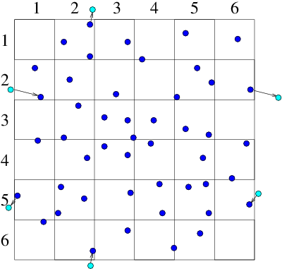
<div style="text-align:center">Figure 10.9: Particles that cross outer periodic boundaries (a) are
    relocated to the opposite side of the domain. This is equivalent (b)
    to modelling an (infinite) periodic array made up of repetitions
    of the smaller domain.<a id="periodicparts">
</a></div>

<div class="p"><!----></div>
Periodic boundaries mean that the computation represents the phenomena
of a periodic array of domains all connected to one another and all
doing the same thing. Sometimes that is actually what one wants. But
more often it is an approximation to a larger domain. If nothing of
interest happens at a scale equal to or larger than the smaller
computational domain, then the artifically imposed periodicity is
unimportant, and the periodic conditions are a convenient way to
represent the computation of a small sub-volume within a much larger,
uniform, medium. Fig.&nbsp;<a href="chap10.xml#periodicparts">10.9</a> illustrates this point.

<div class="p"><!----></div>
Sometimes, however, it is not appropriate to use periodic
conditions. In that case a particle that leaves the domain is simply
removed from the calculation. If the calculation is approximately
steady, then clearly there must also be particles created within the
domain or <em>entering</em> it from outside. A suitable method for
injecting them into the calculation must be implemented. It might
represent, for example, the flux of particles across the boundary from
an assumed velocity distribution function.

<div class="p"><!----></div>

<h2>Worked Example: Required resolution of PIC grid</h2>

<div class="p"><!----></div>
How fine<a 
id="resolution_PIC_mesh102617"></a><a 
id="PIC_resolution102618"></a> must the potential mesh be in an electron Particle in Cell code? 

<div class="p"><!----></div>
<br />Well, it depends on how fine-scale the potential variation might
be. That depends on the parameters of the particles
(electrons). Suppose they have approximately a Maxwell-Boltzmann
velocity-distribution of temperature <math xmlns="http://www.w3.org/1998/Math/MathML">
<mrow>
<msub><mrow><mi>T</mi></mrow><mrow><mi>e</mi></mrow>
</msub>
</mrow></math>. We can estimate the finest
scale of potential variation as follows. We'll consider just a
one-dimensional problem. Suppose there is at some position <math xmlns="http://www.w3.org/1998/Math/MathML">
<mrow><mi>x</mi></mrow></math>, a
perturbed potential <math xmlns="http://www.w3.org/1998/Math/MathML">
<mrow><mi mathvariant="italic">&phi;</mi><mo stretchy="false">(</mo><mi>x</mi><mo stretchy="false">)</mo></mrow></math> such that <math xmlns="http://www.w3.org/1998/Math/MathML">
<mrow><mo stretchy="false">&verbar;</mo><mi mathvariant="italic">&phi;</mi><mo stretchy="false">&verbar;</mo><mo> &lt;&lt; </mo>
<msub><mrow><mi>T</mi></mrow><mrow><mi>e</mi></mrow>
</msub>
<mo stretchy="false">/</mo><mi>e</mi></mrow></math>, measured
from a chosen reference <math xmlns="http://www.w3.org/1998/Math/MathML">
<mrow>
<msub><mrow><mi mathvariant="italic">&phi;</mi></mrow><mrow><mi mathvariant="italic">&infin;</mi></mrow>
</msub>
<mo>=</mo><mn>0</mn></mrow></math> in the equilibrium background
where the density is <math xmlns="http://www.w3.org/1998/Math/MathML">
<mrow>
<msub><mrow><mi>n</mi></mrow><mrow><mi>e</mi></mrow>
</msub>
<mo>=</mo>
<msub><mrow><mi>n</mi></mrow><mrow><mi mathvariant="italic">&infin;</mi></mrow>
</msub>
<mo>=</mo>
<msub><mrow><mi>n</mi></mrow><mrow><mi>i</mi></mrow>
</msub>
</mrow></math>. (Referring to the
background as <math xmlns="http://www.w3.org/1998/Math/MathML">
<mrow><mi mathvariant="italic">&infin;</mi></mrow></math> is a helpful notation that avoids implying the
value at <math xmlns="http://www.w3.org/1998/Math/MathML">
<mrow><mi>x</mi><mo>=</mo><mn>0</mn></mrow></math>; it means the distant value.)  Then the electron
density at <math xmlns="http://www.w3.org/1998/Math/MathML">
<mrow><mi>x</mi></mrow></math> can be deduced from the fact that <math xmlns="http://www.w3.org/1998/Math/MathML">
<mrow><mi>f</mi><mo stretchy="false">(</mo><mi>v</mi><mo stretchy="false">)</mo></mrow></math> is constant along
orbits (characteristics).  In the collisionless steady-state,
energy is conserved; so for any orbit <math xmlns="http://www.w3.org/1998/Math/MathML">
<mrow>
<mfrac><mrow><mn>1</mn></mrow>
<mrow><mn>2</mn></mrow>
</mfrac>

<msup><mrow><mi mathvariant="italic">mv</mi></mrow><mrow><mn>2</mn></mrow>
</msup>
<mo>-</mo><mi>e</mi><mi mathvariant="italic">&phi;</mi><mo>=</mo>
<mfrac><mrow><mn>1</mn></mrow>
<mrow><mn>2</mn></mrow>
</mfrac>

<msubsup><mrow><mi mathvariant="italic">mv</mi></mrow><mrow><mi mathvariant="italic">&infin;</mi> </mrow>
<mrow><mn>2</mn></mrow></msubsup>
</mrow></math>, where <math xmlns="http://www.w3.org/1998/Math/MathML">
<mrow>
<msub><mrow><mi>v</mi></mrow><mrow><mi mathvariant="italic">&infin;</mi></mrow>
</msub>
</mrow></math> is the velocity on that orbit when it
is "at infinity" in the background, where <math xmlns="http://www.w3.org/1998/Math/MathML">
<mrow><mi mathvariant="italic">&phi;</mi><mo>=</mo><mn>0</mn></mrow></math>. Consequently,
<math xmlns="http://www.w3.org/1998/Math/MathML">
<mrow><mi>f</mi><mo stretchy="false">(</mo><mi>v</mi><mo stretchy="false">)</mo><mo>=</mo>
<msub><mrow><mi>f</mi></mrow><mrow><mi mathvariant="italic">&infin;</mi></mrow>
</msub>
<mo stretchy="false">(</mo>
<msub><mrow><mi>v</mi></mrow><mrow><mi mathvariant="italic">&infin;</mi></mrow>
</msub>
<mo stretchy="false">)</mo><mo>=</mo>
<msub><mrow><mi>n</mi></mrow><mrow><mi mathvariant="italic">&infin;</mi></mrow>
</msub>
<msqrt><mrow>
<mfrac><mrow><mi>m</mi></mrow>
<mrow><mn>2</mn><mi mathvariant="italic">&pi;</mi>
<msub><mrow><mi>T</mi></mrow><mrow><mi>e</mi></mrow>
</msub>
</mrow>
</mfrac>
</mrow></msqrt><mi>exp</mi><mo stretchy="false">(</mo><mo>-</mo>
<msubsup><mrow><mi mathvariant="italic">mv</mi></mrow><mrow><mi mathvariant="italic">&infin;</mi> </mrow>
<mrow><mn>2</mn></mrow></msubsup>
<mo stretchy="false">/</mo><mn>2</mn>
<msub><mrow><mi>T</mi></mrow><mrow><mi>e</mi></mrow>
</msub>
<mo stretchy="false">)</mo><mo>=</mo>
<msub><mrow><mi>n</mi></mrow><mrow><mi mathvariant="italic">&infin;</mi></mrow>
</msub>
<msqrt><mrow>
<mfrac><mrow><mi>m</mi></mrow>
<mrow><mn>2</mn><mi mathvariant="italic">&pi;</mi>
<msub><mrow><mi>T</mi></mrow><mrow><mi>e</mi></mrow>
</msub>
</mrow>
</mfrac>
</mrow></msqrt><mi>exp</mi><mo stretchy="false">(</mo><mo>-</mo>
<msup><mrow><mi mathvariant="italic">mv</mi></mrow><mrow><mn>2</mn></mrow>
</msup>
<mo stretchy="false">/</mo><mn>2</mn>
<msub><mrow><mi>T</mi></mrow><mrow><mi>e</mi></mrow>
</msub>
<mo>+</mo><mi>e</mi><mi mathvariant="italic">&phi;</mi><mo stretchy="false">/</mo>
<msub><mrow><mi>T</mi></mrow><mrow><mi>e</mi></mrow>
</msub>
<mo stretchy="false">)</mo></mrow></math>. Hence at <math xmlns="http://www.w3.org/1998/Math/MathML">
<mrow><mi>x</mi></mrow></math>, <math xmlns="http://www.w3.org/1998/Math/MathML">
<mrow><mi>f</mi><mo stretchy="false">(</mo><mi>v</mi><mo stretchy="false">)</mo></mrow></math> is Maxwellian with density
<math xmlns="http://www.w3.org/1998/Math/MathML">
<mrow><mi>n</mi><mo>=</mo><mo>&int;</mo><mi>f</mi><mo stretchy="false">(</mo><mi>v</mi><mo stretchy="false">)</mo><mi mathvariant="italic">dv</mi><mo>=</mo>
<msub><mrow><mi>n</mi></mrow><mrow><mi mathvariant="italic">&infin;</mi></mrow>
</msub>
<mi>exp</mi><mo stretchy="false">(</mo><mi>e</mi><mi mathvariant="italic">&phi;</mi><mo stretchy="false">/</mo>
<msub><mrow><mi>T</mi></mrow><mrow><mi>e</mi></mrow>
</msub>
<mo stretchy="false">)</mo></mrow></math>.

<div class="p"><!----></div>
Now let's find analytically the steady potential arising for <math xmlns="http://www.w3.org/1998/Math/MathML">
<mrow><mi>x</mi><mo>&gt;</mo><mn>0</mn></mrow></math> when the
potential slope at <math xmlns="http://www.w3.org/1998/Math/MathML">
<mrow><mi>x</mi><mo>=</mo><mn>0</mn></mrow></math> is <math xmlns="http://www.w3.org/1998/Math/MathML">
<mrow><mi>d</mi><mi mathvariant="italic">&phi;</mi><mo stretchy="false">/</mo><mi mathvariant="italic">dx</mi><mo>=</mo><mo>-</mo>
<msub><mrow><mi>E</mi></mrow><mrow><mn>0</mn></mrow>
</msub>
</mrow></math>. Poisson's equation in
one-dimension is 
<a id="wk10eq1">
</a><br />
<table width="100%"><tr><td align="center">
    <math xmlns="http://www.w3.org/1998/Math/MathML">
    <mstyle displaystyle="true"><mrow>
<mfrac><mrow>
<msup><mrow><mi>d</mi></mrow><mrow><mn>2</mn></mrow>
</msup>
<mi mathvariant="italic">&phi;</mi></mrow>
<mrow>
<msup><mrow><mi mathvariant="italic">dx</mi></mrow><mrow><mn>2</mn></mrow>
</msup>
</mrow>
</mfrac>
<mo>=</mo><mo>-</mo>
<mfrac><mrow>
<msub><mrow><mi mathvariant="italic">en</mi></mrow><mrow><mi mathvariant="italic">&infin;</mi></mrow>
</msub>
</mrow>
<mrow>
<msub><mrow><mi mathvariant="italic">&epsi;</mi></mrow><mrow><mn>0</mn></mrow>
</msub>
</mrow>
</mfrac>
<mrow><mo>[</mo><mn>1</mn><mo>-</mo><mi>exp</mi><mo stretchy="false">(</mo><mi>e</mi><mi mathvariant="italic">&phi;</mi><mo stretchy="false">/</mo>
<msub><mrow><mi>T</mi></mrow><mrow><mi>e</mi></mrow>
</msub>
<mo stretchy="false">)</mo><mo>]</mo></mrow><mo>&ap;</mo><mrow><mo>(</mo>
<mfrac><mrow>
<msup><mrow><mi>e</mi></mrow><mrow><mn>2</mn></mrow>
</msup>

<msub><mrow><mi>n</mi></mrow><mrow><mi mathvariant="italic">&infin;</mi></mrow>
</msub>
</mrow>
<mrow>
<msub><mrow><mi mathvariant="italic">&epsi;</mi></mrow><mrow><mn>0</mn></mrow>
</msub>

<msub><mrow><mi>T</mi></mrow><mrow><mi>e</mi></mrow>
</msub>
</mrow>
</mfrac>
<mo>)</mo></mrow><mi mathvariant="italic">&phi;</mi><mo>.</mo></mrow>
    </mstyle></math></td><td width="1">
    <math xmlns="http://www.w3.org/1998/Math/MathML">
    <mstyle displaystyle="true"><mrow><mo stretchy="false">(</mo><mn>10</mn><mo>.</mo><mn>7</mn><mo stretchy="false">)</mo></mrow>
    </mstyle></math>
</td></tr></table>


The final approximate form gives Helmholtz's equation. It is obtained by
Taylor expansion of the exponential to first order, since its argument
is small. The solution satisfying the condition at <math xmlns="http://www.w3.org/1998/Math/MathML">
<mrow><mi>x</mi><mo>=</mo><mn>0</mn></mrow></math> is then
<a id="wk10eq2">
</a><br />
<table width="100%"><tr><td align="center">
    <math xmlns="http://www.w3.org/1998/Math/MathML">
    <mstyle displaystyle="true"><mrow><mi mathvariant="italic">&phi;</mi><mo stretchy="false">(</mo><mi>x</mi><mo stretchy="false">)</mo><mo>=</mo>
<msub><mrow><mi>E</mi></mrow><mrow><mn>0</mn></mrow>
</msub>
<mi mathvariant="italic">&lambda;</mi>
<msup><mrow><mi fontstyle="normal">e</mi></mrow><mrow><mo>-</mo><mi>x</mi><mo stretchy="false">/</mo><mi mathvariant="italic">&lambda;</mi></mrow>
</msup>
<mo>,</mo><mi>&emsp;&emsp;&emsp;</mi>
<mtext>where</mtext>
<mi>&emsp;&emsp;&emsp;</mi>
<msup><mrow><mi mathvariant="italic">&lambda;</mi></mrow><mrow><mn>2</mn></mrow>
</msup>
<mo>=</mo><mrow><mo>(</mo>
<mfrac><mrow>
<msup><mrow><mi>e</mi></mrow><mrow><mn>2</mn></mrow>
</msup>

<msub><mrow><mi>n</mi></mrow><mrow><mi mathvariant="italic">&infin;</mi></mrow>
</msub>
</mrow>
<mrow>
<msub><mrow><mi mathvariant="italic">&epsi;</mi></mrow><mrow><mn>0</mn></mrow>
</msub>

<msub><mrow><mi>T</mi></mrow><mrow><mi>e</mi></mrow>
</msub>
</mrow>
</mfrac>
<mo>)</mo></mrow><mo>.</mo></mrow>
    </mstyle></math></td><td width="1">
    <math xmlns="http://www.w3.org/1998/Math/MathML">
    <mstyle displaystyle="true"><mrow><mo stretchy="false">(</mo><mn>10</mn><mo>.</mo><mn>8</mn><mo stretchy="false">)</mo></mrow>
    </mstyle></math>
</td></tr></table>


Based on this model calculation, the length
<math xmlns="http://www.w3.org/1998/Math/MathML">
<mrow><mi mathvariant="italic">&lambda;</mi><mo>=</mo><msqrt><mrow>
<msup><mrow><mi>e</mi></mrow><mrow><mn>2</mn></mrow>
</msup>

<msub><mrow><mi>n</mi></mrow><mrow><mi mathvariant="italic">&infin;</mi></mrow>
</msub>
<mo stretchy="false">/</mo>
<msub><mrow><mi mathvariant="italic">&epsi;</mi></mrow><mrow><mn>0</mn></mrow>
</msub>

<msub><mrow><mi>T</mi></mrow><mrow><mi>e</mi></mrow>
</msub>
</mrow></msqrt></mrow></math>, which is called the Debye
length<a 
id="Debye_length102619"></a>, is the characteristic spatial scale of
potential variation. A PIC calculation must have fine enough grid to
resolve the smaller of <math xmlns="http://www.w3.org/1998/Math/MathML">
<mrow><mi mathvariant="italic">&lambda;</mi></mrow></math> and the characteristic feature-size
of any object in the problem whose influence introduces potential
structure. In short, <math xmlns="http://www.w3.org/1998/Math/MathML">
<mrow><mi mathvariant="italic">&Delta;</mi><mi>x</mi><mo>&le;</mo><mi mathvariant="italic">&lambda;</mi></mrow></math>.

<div class="p"><!----></div>
If we had an operational PIC code, we could do a series of
calculations with different cell size <math xmlns="http://www.w3.org/1998/Math/MathML">
<mrow><mi mathvariant="italic">&Delta;</mi><mi>x</mi></mrow></math>. We would find that
when <math xmlns="http://www.w3.org/1998/Math/MathML">
<mrow><mi mathvariant="italic">&Delta;</mi><mi>x</mi></mrow></math> became small enough, the solutions would give a result
independent of <math xmlns="http://www.w3.org/1998/Math/MathML">
<mrow><mi mathvariant="italic">&Delta;</mi><mi>x</mi></mrow></math>. That would be a good way of demonstrating
adequate spatial resolution<a 
id="spatial_resolution102620"></a> numerically. For
the simple problem we've considered the requirement can be calculated
analytically. Actually the criterion <math xmlns="http://www.w3.org/1998/Math/MathML">
<mrow><mi mathvariant="italic">&Delta;</mi><mi>x</mi><mo>&lt;~</mo><mi mathvariant="italic">&lambda;</mi></mrow></math> applies
very widely in plasma PIC calculations.

<div class="p"><!----></div>

<h2>Exercise 10. Atomistic Simulation</h2>

<div class="p"><!----></div>
<br /><br />1. The Verlet scheme for particle advance is
<br />
<table width="100%"><tr><td align="center">
    <math xmlns="http://www.w3.org/1998/Math/MathML">
    <mstyle displaystyle="true"><mrow>
<mtable displaystyle="true" align="right" width="80%">
<mtr><mtd columnalign="right" columnspan="1"><mrow>
<msub><mrow><mi mathvariant="bold-italic">x</mi></mrow><mrow><mi>n</mi><mo>+</mo><mn>1</mn></mrow>
</msub>
</mrow>
</mtd><mtd columnalign="left">
<mrow><mo>=</mo></mrow>
</mtd><mtd columnalign="left">
<mrow>
<msub><mrow><mi mathvariant="bold-italic">x</mi></mrow><mrow><mi>n</mi></mrow>
</msub>
<mo>+</mo>
<msub><mrow><mi mathvariant="bold-italic">v</mi></mrow><mrow><mi>n</mi></mrow>
</msub>
<mi mathvariant="italic">&Delta;</mi><mi>t</mi><mo>+</mo>
<msub><mrow><mi mathvariant="bold-italic">a</mi></mrow><mrow><mi>n</mi></mrow>
</msub>
<mi mathvariant="italic">&Delta;</mi>
<msup><mrow><mi>t</mi></mrow><mrow><mn>2</mn></mrow>
</msup>
<mo stretchy="false">/</mo><mn>2</mn></mrow>
</mtd></mtr>
<mtr><mtd columnalign="right" columnspan="1"><mrow>
<msub><mrow><mi mathvariant="bold-italic">v</mi></mrow><mrow><mi>n</mi><mo>+</mo><mn>1</mn></mrow>
</msub>
</mrow>
</mtd><mtd columnalign="left">
<mrow><mo>=</mo></mrow>
</mtd><mtd columnalign="left">
<mrow>
<msub><mrow><mi mathvariant="bold-italic">v</mi></mrow><mrow><mi>n</mi></mrow>
</msub>
<mo>+</mo><mo stretchy="false">(</mo>
<msub><mrow><mi mathvariant="bold-italic">a</mi></mrow><mrow><mi>n</mi></mrow>
</msub>
<mo>+</mo>
<msub><mrow><mi mathvariant="bold-italic">a</mi></mrow><mrow><mi>n</mi><mo>+</mo><mn>1</mn></mrow>
</msub>
<mo stretchy="false">)</mo><mi mathvariant="italic">&Delta;</mi><mi>t</mi><mo stretchy="false">/</mo><mn>2</mn><mo>.</mo></mrow>
</mtd><mtd columnalign="right">&emsp;&emsp;&emsp;&emsp;&emsp;&emsp;<mo stretchy="false">(</mo><mn>10</mn><mo>.</mo><mn>9</mn><mo stretchy="false">)</mo></mtd></mtr>
</mtable>
</mrow>
    </mstyle></math>
</td></tr></table>
<br />

Suppose that the velocity at integer timesteps is related to that at
half integer timesteps by
<math xmlns="http://www.w3.org/1998/Math/MathML">
<mrow>
<msub><mrow><mi mathvariant="bold-italic">v</mi></mrow><mrow><mi>n</mi></mrow>
</msub>
<mo>=</mo><mo stretchy="false">(</mo>
<msub><mrow><mi mathvariant="bold-italic">v</mi></mrow><mrow><mi>n</mi><mo>-</mo><mn>1</mn><mo stretchy="false">/</mo><mn>2</mn></mrow>
</msub>
<mo>+</mo>
<msub><mrow><mi mathvariant="bold-italic">v</mi></mrow><mrow><mi>n</mi><mo>+</mo><mn>1</mn><mo stretchy="false">/</mo><mn>2</mn></mrow>
</msub>
<mo stretchy="false">)</mo><mo stretchy="false">/</mo><mn>2</mn></mrow></math>.
With this identification, derive the Verlet scheme from
the leap-frog scheme,
<br />
<table width="100%"><tr><td align="center">
    <math xmlns="http://www.w3.org/1998/Math/MathML">
    <mstyle displaystyle="true"><mrow>
<mtable displaystyle="true" align="right" width="80%">
<mtr><mtd columnalign="right" columnspan="1"><mrow>
<msub><mrow><mi mathvariant="bold-italic">x</mi></mrow><mrow><mi>n</mi><mo>+</mo><mn>1</mn></mrow>
</msub>
</mrow>
</mtd><mtd columnalign="left">
<mrow><mo>=</mo></mrow>
</mtd><mtd columnalign="left">
<mrow>
<msub><mrow><mi mathvariant="bold-italic">x</mi></mrow><mrow><mi>n</mi></mrow>
</msub>
<mo>+</mo>
<msub><mrow><mi mathvariant="bold-italic">v</mi></mrow><mrow><mi>n</mi><mo>+</mo><mn>1</mn><mo stretchy="false">/</mo><mn>2</mn></mrow>
</msub>
<mi mathvariant="italic">&Delta;</mi><mi>t</mi></mrow>
</mtd></mtr>
<mtr><mtd columnalign="right" columnspan="1"><mrow>
<msub><mrow><mi mathvariant="bold-italic">v</mi></mrow><mrow><mi>n</mi><mo>+</mo><mn>3</mn><mo stretchy="false">/</mo><mn>2</mn></mrow>
</msub>
</mrow>
</mtd><mtd columnalign="left">
<mrow><mo>=</mo></mrow>
</mtd><mtd columnalign="left">
<mrow>
<msub><mrow><mi mathvariant="bold-italic">v</mi></mrow><mrow><mi>n</mi><mo>+</mo><mn>1</mn><mo stretchy="false">/</mo><mn>2</mn></mrow>
</msub>
<mo>+</mo>
<msub><mrow><mi mathvariant="bold-italic">a</mi></mrow><mrow><mi>n</mi><mo>+</mo><mn>1</mn></mrow>
</msub>
<mi mathvariant="italic">&Delta;</mi><mi>t</mi><mo>,</mo></mrow>
</mtd><mtd columnalign="right">&emsp;&emsp;&emsp;&emsp;&emsp;&emsp;<mo stretchy="false">(</mo><mn>10</mn><mo>.</mo><mn>10</mn><mo stretchy="false">)</mo></mtd></mtr>
</mtable>
</mrow>
    </mstyle></math>
</td></tr></table>
<br />

and thus show they are equivalent.

<div class="p"><!----></div>
<br /><br /> 2. A block algorithm is applied to an atomistic
simulation in a cubical 3 dimensional region, containing <math xmlns="http://www.w3.org/1998/Math/MathML">
<mrow>
<msub><mrow><mi>N</mi></mrow><mrow><mi>p</mi></mrow>
</msub>
<mo>=</mo><mn>1000000</mn></mrow></math>
atoms approximately uniformly distributed. Only two-particle forces
are to be considered. The cut-off range for particle-particle force is
4 times the average particle spacing. Find

<div class="p"><!----></div>
(a) The optimal size of blocks into which to divide the domain for
fastest execution.

<div class="p"><!----></div>
(b) How many force evaluations per time-step will be required.

<div class="p"><!----></div>
(c) If the force evaluations require 5 multiplications, a Verlet
advance is used, and the calculation is done on a single processor
which takes 1 nanosecond per multiplication on average, roughly what
is the total time taken per timestep (for the full 1,000,000 particles).

<div class="p"><!----></div>
<br /><br /> 3. (a) Prove from the definition of a characteristic
(see section <a href="chap8.xml#characteristicsec">8.3.2</a>) that the equation of the
characteristics of the collisionless Boltzmann equation is
<br />
<table width="100%"><tr><td align="center">
    <math xmlns="http://www.w3.org/1998/Math/MathML">
    <mstyle displaystyle="true"><mrow>
<mfrac><mrow><mi>d</mi></mrow>
<mrow><mi mathvariant="italic">dt</mi></mrow>
</mfrac>
<mrow><mo>(</mo>
<mfrac linethickness="0"><mrow><mi mathvariant="bold-italic">x</mi></mrow>
<mrow><mi mathvariant="bold-italic">v</mi></mrow>
</mfrac>
<mo>)</mo></mrow><mo>=</mo><mrow><mo>(</mo>
<mfrac linethickness="0"><mrow><mi mathvariant="bold-italic">v</mi></mrow>
<mrow><mi mathvariant="bold-italic">a</mi></mrow>
</mfrac>
<mo>)</mo></mrow><mo>.</mo></mrow>
    </mstyle></math></td><td width="1">
    <math xmlns="http://www.w3.org/1998/Math/MathML">
    <mstyle displaystyle="true"><mrow><mo stretchy="false">(</mo><mn>10</mn><mo>.</mo><mn>11</mn><mo stretchy="false">)</mo></mrow>
    </mstyle></math>
</td></tr></table>


Show also that a particle (or pseudo-particle) trajectory in a fixed
electric potential depends only on initial velocity and the ratio of
its charge to mass <math xmlns="http://www.w3.org/1998/Math/MathML">
<mrow><mi>q</mi><mo stretchy="false">/</mo><mi>m</mi></mrow></math>, and therefore that the equation of motion of
a pseudo-particle must use the same <math xmlns="http://www.w3.org/1998/Math/MathML">
<mrow><mi>q</mi><mo stretchy="false">/</mo><mi>m</mi></mrow></math> as the actual particles, if
a PIC simulation is to model correctly the force law at given speed
and potential.

<div class="p"><!----></div>
(b) A pseudo-particle of charge <math xmlns="http://www.w3.org/1998/Math/MathML">
<mrow><mi>q</mi></mrow></math> follows a characteristic, but it
is supposed to be representative of many nearby particles
(characteristics). If the mean density of pseudo-particles in a PIC
simulation is a factor <math xmlns="http://www.w3.org/1998/Math/MathML">
<mrow><mn>1</mn><mo stretchy="false">/</mo><mi>g</mi></mrow></math> (where <math xmlns="http://www.w3.org/1998/Math/MathML">
<mrow><mi>g</mi><mo>&gt;&gt;</mo><mn>1</mn></mrow></math>) smaller than the actual
density of the system being modelled, how much charge must each
pseudo-particle deposit on the potential grid to give the correct
potential from Poisson's equation? One way to do PIC simulation is to
represent all lengths, times, charges and masses in physical units,
but to use this charge deposition factor, and correspondingly lower
particle density.

<div class="p"><!----></div>


<hr /><table width="100%"><tr><td>
 <a href="index.xml">HEAD</a></td><td align="right">
<a href="chap11.xml">NEXT
</a></td></tr></table>
</div></body></html>